Working with time in Xarray

Sign up to the DEA Sandbox to run this notebook interactively from a browser
Compatibility: Notebook currently compatible with both the NCI and DEA Sandbox environments
Products used: ga_ls8c_ard_3

Description

The xarray Python package provides many useful techniques for dealing with time series data that can be applied to Digital Earth Australia data. This notebook demonstrates how to use xarray techniques to:

Select different time periods of data (e.g. year, month, day) from an xarray.Dataset
Using datetime accessors to extract additional information from a dataset’s time dimension
Summarising time series data for different time periods using .groupby() and .resample()
Interpolating time series data to estimate landscape conditions at a specific date that the satellite did not observe

For additional information about the techniques demonstrated below, refer to the xarray Time series data guide.

Getting started

To run this analysis, run all the cells in the notebook, starting with the “Load packages” cell.

Load packages

[1]:

%matplotlib inline

import datacube
import matplotlib.pyplot as plt

Connect to the datacube

[2]:

dc = datacube.Datacube(app='Working_with_time')

Loading Landsat data

First, we load in a two years of Landsat 8 data, and apply a simple cloud mask. To learn more about masking data, see the masking data notebook.

[3]:

# Set up a location for the analysis
query = {
    'x': (142.41, 142.51),
    'y': (-32.22, -32.32),
    'time': ('2015-01-01', '2016-12-31'),
    'measurements': ['nbart_nir', 'fmask'],
    'output_crs': 'EPSG:3577',
    'resolution': (-30, 30)
}

# Load Landsat 8 data
ds = dc.load(product='ga_ls8c_ard_3', group_by='solar_day', **query)

# Apply simple cloud mask (keep only clear, water or snow observations)
ds = ds.where(ds.fmask.isin([1, 4, 5]))

print(ds)

<xarray.Dataset>
Dimensions:      (time: 46, x: 342, y: 398)
Coordinates:
  * time         (time) datetime64[ns] 2015-01-06T00:20:26.943424 ... 2016-12...
  * y            (y) float64 -3.552e+06 -3.552e+06 ... -3.563e+06 -3.563e+06
  * x            (x) float64 9.709e+05 9.71e+05 9.71e+05 ... 9.811e+05 9.812e+05
    spatial_ref  int32 3577
Data variables:
    nbart_nir    (time, y, x) float64 nan nan nan nan nan ... nan nan nan nan
    fmask        (time, y, x) float64 nan nan nan nan nan ... nan nan nan nan
Attributes:
    crs:           EPSG:3577
    grid_mapping:  spatial_ref

Working with time

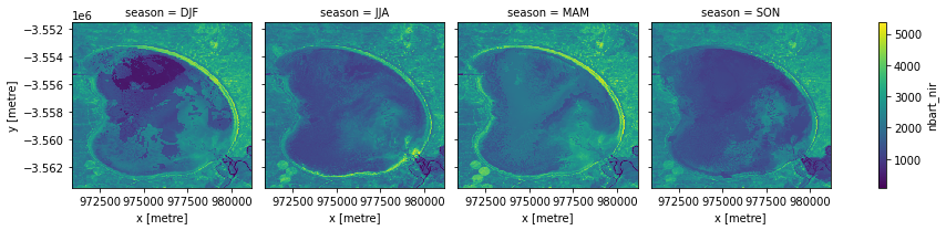
Grouping and resampling by time

xarray also provides some shortcuts for aggregating data over time. In the example below, we first group our data by season, then take the median of each group. This produces a new dataset with only four observations (one per season).

[9]:

# Group the time series into seasons, and take median of each time period
ds_seasonal = ds.groupby('time.season').median(dim='time')

# Plot the output
ds_seasonal.nbart_nir.plot(col='season', col_wrap=4)
plt.show()

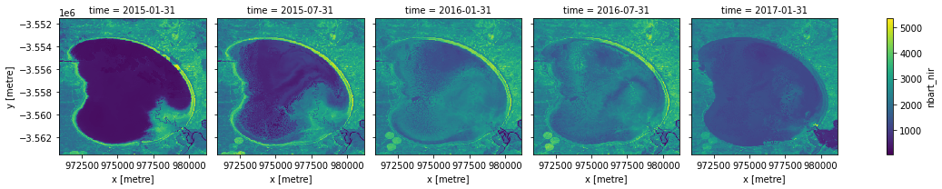
../../../_images/notebooks_How_to_guides_Working_with_time_20_0.png

We can also use the .resample() method to summarise our dataset into larger chunks of time. In the example below, we produce a median composite for every 6 months of data in our dataset:

[10]:

# Resample to combine each 6 months of data into a median composite
ds_resampled = ds.resample(time='6m').median()

# Plot the new resampled data
ds_resampled.nbart_nir.plot(col='time')
plt.show()

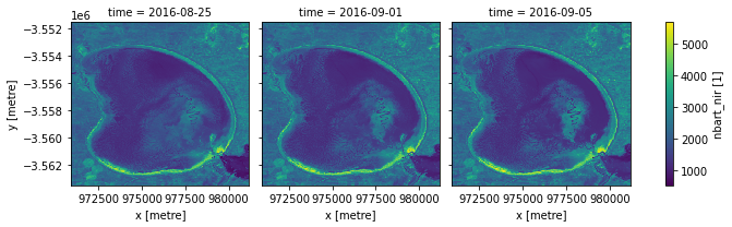
../../../_images/notebooks_How_to_guides_Working_with_time_22_0.png

Interpolating new timesteps

Sometimes, we want to return data for specific times/dates that weren’t observed by a satellite. To estimate what the landscape appeared like on certain dates, we can use the .interp() method to interpolate between the nearest two observations.

By default, the interp() method uses linear interpolation (method='linear'). Another useful option is method='nearest', which will return the nearest satellite observation to the specified date(s).

[11]:

# New dates to interpolate data for
new_dates = ['2016-08-25', '2016-09-01', '2016-09-05']

# Interpolate Landsat values for three new dates
ds_interp = ds.interp(time=new_dates)

# Plot the new interpolated data
ds_interp.nbart_nir.plot(col='time')
plt.show()

../../../_images/notebooks_How_to_guides_Working_with_time_24_0.png

Additional information

License: The code in this notebook is licensed under the Apache License, Version 2.0. Digital Earth Australia data is licensed under the Creative Commons by Attribution 4.0 license.

Contact: If you need assistance, please post a question on the Open Data Cube Slack channel or on the GIS Stack Exchange using the open-data-cube tag (you can view previously asked questions here). If you would like to report an issue with this notebook, you can file one on GitHub.

Last modified: December 2023

Compatible datacube version:

[12]:

print(datacube.__version__)

1.8.5