Introduction to DEA Coastlines

Sign up to the DEA Sandbox to run this notebook interactively from a browser
Compatibility: Notebook currently compatible with both the NCI and DEA Sandbox environments
Products used: DEA Coastlines

Background

Australia has a highly dynamic coastline of over 30,000 km, with over 85% of its population living within 50 km of the coast. This coastline is subject to a wide range of pressures, including extreme weather and climate, sea level rise and human development. Understanding how the coastline responds to these pressures is crucial to managing this region, from social, environmental and economic perspectives.

What this product offers

Digital Earth Australia Coastlines is a continental dataset that includes annual shorelines and rates of coastal change along the entire Australian coastline from 1988 to the present.

The product combines satellite data from Geoscience Australia’s Digital Earth Australia program with tidal modelling to map the typical location of the coastline at mean sea level for each year. The product enables trends of coastal erosion and growth to be examined annually at both a local and continental scale, and for patterns of coastal change to be mapped historically and updated regularly as data continues to be acquired. This allows current rates of coastal change to be compared with that observed in previous years or decades.

The ability to map shoreline positions for each year provides valuable insights into whether changes to our coastline are the result of particular events or actions, or a process of more gradual change over time. This information can enable scientists, managers and policy makers to assess impacts from the range of drivers impacting our coastlines and potentially assist planning and forecasting for future scenarios.

Applications

Monitoring and mapping rates of coastal erosion along the Australian coastline
Prioritise and evaluate the impacts of local and regional coastal management based on historical coastline change
Modelling how coastlines respond to drivers of change, including extreme weather events, sea level rise or human development
Supporting geomorphological studies of how and why coastlines have changed across time

Publications

Bishop-Taylor, R., Nanson, R., Sagar, S., Lymburner, L. (2021). Mapping Australia’s dynamic coastline at mean sea level using three decades of Landsat imagery. Remote Sensing of Environment, 267, 112734. Available: https://doi.org/10.1016/j.rse.2021.112734
Nanson, R., Bishop-Taylor, R., Sagar, S., Lymburner, L., (2022). Geomorphic insights into Australia’s coastal change using a national dataset derived from the multi-decadal Landsat archive. Estuarine, Coastal and Shelf Science, 265, p.107712. Available: https://doi.org/10.1016/j.ecss.2021.107712
Bishop-Taylor, R., Sagar, S., Lymburner, L., Alam, I., & Sixsmith, J. (2019). Sub-pixel waterline extraction: Characterising accuracy and sensitivity to indices and spectra. Remote Sensing, 11(24), 2984. Available: https://www.mdpi.com/2072-4292/11/24/2984

Note: For more technical information about the DEA Coastlines product, visit the official Geoscience Australia DEA Coastlines product description.. To explore DEA Coastlines on an interactive map, visit DEA Maps.

Description

This notebook will demonstrate how to load data from the Digital Earth Australia Coastlines product using the Digital Earth Australia datacube. Topics covered include:

Loading DEA Coastlines annual shoreline data using the get_coastlines function.
Loading DEA Coastlines rates of change statistics data using the get_coastlines function.

Getting started

To run this analysis, run all the cells in the notebook, starting with the “Load packages” cell.

Load packages

[1]:

import geopandas as gpd
import matplotlib.pyplot as plt

import sys
sys.path.insert(1, '../Tools/')
from dea_tools.coastal import get_coastlines

Loading DEA Coastlines data

Annual shorelines

DEA Coastlines data can be loaded directly in a Python script or Jupyter Notebook using the DEA Coastlines Web Feature Service (WFS) and geopandas:

[2]:

# Specify bounding box
ymax, xmin = -33.65, 115.28
ymin, xmax = -33.66, 115.30

# Load DEA Coastlines annual shorelines data
deacl_annualshorelines_gdf = get_coastlines(bbox=(xmin, ymin, xmax, ymax),
                                      layer='shorelines_annual')

# Print example output
deacl_annualshorelines_gdf.head()

[2]:

	id	year	certainty	tide_datum	id_primary	geometry
37	shorelines_annual.29704	1990	unstable data	0.0 m AMSL	WA12	MULTILINESTRING ((-1536327.590 -3772770.634, -...
46	shorelines_annual.29713	2012	good	0.0 m AMSL	WA12	LINESTRING (-1536001.512 -3772716.097, -153601...
45	shorelines_annual.29712	1995	good	0.0 m AMSL	WA12	LINESTRING (-1536001.512 -3772710.925, -153601...
49	shorelines_annual.29716	1994	good	0.0 m AMSL	WA12	LINESTRING (-1536001.512 -3772711.869, -153601...
42	shorelines_annual.29709	2013	good	0.0 m AMSL	WA12	LINESTRING (-1536001.512 -3772715.520, -153601...

We can now plot the DEA Coastlines annual shoreline data using geopandas. Zoom in to Bussleton in Western Australia on the interactive map to view the shoreline data.

Annual shorelines represent the median or ‘most representative’ position of the shoreline at approximately mean sea level tide (0 m Above Mean Sea Level) for each year from 1988 onward. Light-coloured lines (e.g. yellow) in the plot below represent recent shorelines, and dark-coloured lines represent older shorelines (e.g. 1988).

Note: For more detail about DEA Coastlines annual shoreline data, refer to the official Geoscience Australia DEA Coastlines product description.

[3]:

# Plot on interactive map of DEA Coastlines data within our bounding box
deacl_annualshorelines_gdf.explore(column='year', cmap='inferno', categorical=True)

[3]:

Make this Notebook Trusted to load map: File -> Trust Notebook

Rates of change points

We can also load and plot the DEA Coastlines rates of change points. These points provide robust rates of annual coastal change (in metres per year) for every 30 m along Australia’s non-rocky (e.g. sandy and muddy) coastlines. These rates are calculated by linearly regressing annual shoreline positions against time, using the most recent shoreline as a baseline.

The DEA Coastlines rates of change points data provides many useful statistics that give insights into coastal change in Australia.

Note: For a full description of each of these statistics, refer to the Rates of change section of the official Geoscience Australia DEA Coastlines product description.

[4]:

# Load DEA Coastlines rates of change points within our bounding box
deacl_ratesofchange_gdf = get_coastlines(
    bbox=(xmin, ymin, xmax, ymax), layer="rates_of_change"
)

# Filter points to statistically significant results only (p <= 0.01),
# and points with good certainty (i.e. no poor quality flags)
deacl_ratesofchange_gdf = deacl_ratesofchange_gdf.query("sig_time <= 0.01")
deacl_ratesofchange_gdf = deacl_ratesofchange_gdf.query("certainty == 'good'")

# Print output
deacl_ratesofchange_gdf.head()

[4]:

	id	uid	rate_time	se_time	outl_time	dist_1988	dist_1989	dist_1990	dist_1991	...	angle_std	valid_obs	valid_span	sce	nsm	max_year	min_year	certainty	id_primary	geometry
1	rates_of_change.1571088	qd1bx31g28	-5.19	0.27	None	139.51	136.20	132.94	130.16	...	7	34	34	142.61	-139.51	1988	2012	good	WA12	POINT (-1537098.291 -3773092.096)
3	rates_of_change.1571091	qd1bx31e97	-4.77	0.26	None	128.19	125.07	123.13	119.32	...	11	34	34	132.21	-128.19	1988	2012	good	WA12	POINT (-1537127.839 -3773089.419)
0	rates_of_change.1571087	qd1bx3450p	-5.43	0.28	None	141.49	137.89	137.74	135.67	...	8	34	34	144.33	-141.49	1988	2014	good	WA12	POINT (-1537068.853 -3773088.742)
8	rates_of_change.1571098	qd1bx31k41	-4.19	0.23	None	113.13	113.70	108.17	103.91	...	17	34	34	117.01	-113.13	1989	2016	good	WA12	POINT (-1537157.089 -3773084.735)
2	rates_of_change.1571090	qd1bx345rx	-5.51	0.29	None	137.32	134.05	133.22	131.22	...	9	34	34	143.96	-137.32	1988	2017	good	WA12	POINT (-1537040.291 -3773080.355)

5 rows × 51 columns

Negative rates of change (red points) on the map below indicate retreat (e.g. erosion), and positive values indicate growth (e.g. progradation) over time. By default, rates of change are shown for good quality points with a statistically significant trend over time only.

[5]:

# Add human-friendly label for plotting
deacl_ratesofchange_gdf["Coastal change"] = deacl_ratesofchange_gdf.apply(
    lambda x: f'<h4>This coastline has {"<b>retreated</b>" if x.rate_time < 0 else "<b>grown</b>"} '
    f"by</br><b>{x.rate_time:.2f} m (±{x.se_time * 1.96:.1f}) per year</b> since <b>1988</b></h4>",
    axis=1,
)

# Plot on interactive map
deacl_ratesofchange_gdf.explore(
    column="rate_time", cmap="RdBu", vmin=-3, vmax=3, tooltip="Coastal change"
)

[5]:

Make this Notebook Trusted to load map: File -> Trust Notebook

Exporting DEA Coastlines data as vector files

We can easily export the loaded data as spatial vector files (e.g. ESRI Shapefiles or GeoJSON) so that they can be analysed further in GIS software:

[6]:

deacl_annualshorelines_gdf.to_file('deacoastlines_shorelines.shp')
deacl_ratesofchange_gdf.to_file('deacoastlines_statistics.shp')

/tmp/ipykernel_658/1542491713.py:2: UserWarning: Column names longer than 10 characters will be truncated when saved to ESRI Shapefile.
  deacl_ratesofchange_gdf.to_file('deacoastlines_statistics.shp')

Next steps

DEA Coastlines analysis tools

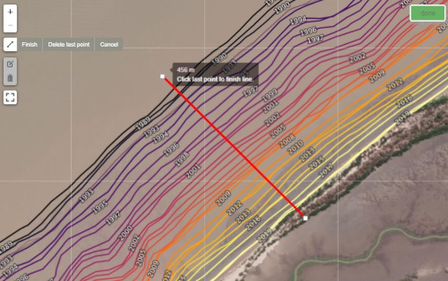
The Coastal transect interactive app allows you to analyse DEA Coastlines data directly in the DEA Sandbox without having to download data to your desktop or use a GIS.

The interactive app can be used to draw transects on the map, and use these to track how a coastline has changed over recent decades. Existing transects (i.e. in Esri Shapefile or GeoJSON format) can also be uploaded directly into the tool, and outputs can be exported as both figures and raw CSVs containing shoreline positions for each year since 1988.

Transect example

Coastline erosion notebook

The Coastal erosion notebook in this repository provides a simplified example of the method used to extract DEA Coastlines annual shoreline data. Run this notebook if you would like to generate more customised coastlines for a specific location, time period, epoch (e.g. annual or biennial coastlines) or tidal range (e.g. the position of the coastline at low, mid or high tide).

Note: This notebook currently supports extracting coastline data only, not generating rates of change statistics like those included in the DEA Coastlines product.

Additional information

License: The code in this notebook is licensed under the Apache License, Version 2.0. Digital Earth Australia data is licensed under the Creative Commons by Attribution 4.0 license.

Contact: If you need assistance, please post a question on the Open Data Cube Slack channel or on the GIS Stack Exchange using the open-data-cube tag (you can view previously asked questions here). If you would like to report an issue with this notebook, you can file one on GitHub.

Last modified: December 2023