Introduction to DEA High and Low Tide Imagery

Sign up to the DEA Sandbox to run this notebook interactively from a browser
Compatibility: Notebook currently compatible with both the NCI and DEA Sandbox environments
Products used: high_tide_comp_20p, low_tide_comp_20p

Background

Intertidal zones are those which are exposed to the air at low tide and underwater at high tide. These include sandy beaches, tidal flats, rocky shores and reefs.

Intertidal zones form critical habitats for a wide range of organisms, but are faced with increasing threats, including coastal erosion and a rise in sea levels.

The ever-changing nature of the tides makes it hard to systematically capture consistent imagery of the intertidal zone, particularly across large regions. Pressure is mounting on this zone from sea-level rise and anthropogenic sources such as land reclamation and aquaculture.

What this product offers

The DEA High and Low Tide Imagery product is a suite of cloud-free composite imagery of the intertidal zones at high and low tide around the Australian coast. It calculates the geometric median (geomedian) of the highest and lowest 20% of the observed tidal range in Digital Earth Australia (DEA)’s archive of Landsat satellite images.

To generate these composites, the archive of Landsat images has been paired with regional tidal modelling, generated by Oregon State Tidal Prediction software. This allows the archive to be sorted by tide height rather than date, so the intertidal zone can be visualised at any stage of the tide regime.

The data has been captured on a 25m spatial scale.

Applications

Mapping cover types within the intertidal zone
Visualising the full observed extent of the tidal range around the Australian continental coastline

Publications

Sagar, S., Phillips, C., Bala, B., Roberts, D., & Lymburner, L. (2018). Generating continental scale pixel-based surface reflectance composites in coastal regions with the use of a multi-resolution tidal model. Remote Sensing, 10(3), 480.

Note: For more technical information about DEA High and Low Tide Imagery, visit the official Geoscience Australia DEA High and Low Tide Imagery product description.

Description

This notebook will demonstrate how to load data from the DEA High and Low Tide product suite using the Digital Earth Australia datacube. Topics covered include:

Inspecting the products and measurements available in the datacube
Loading low and high tide data for a coastal location
Plotting low and high tide data in true and false colour
Converting low and high tide data to a remote sensing water index (NDWI), and use this to map wet pixels at low and high tide

Getting started

To run this analysis, run all the cells in the notebook, starting with the “Load packages” cell.

Load packages

Import Python packages that are used for the analysis.

[1]:

import datacube
import matplotlib.pyplot as plt

import sys
sys.path.insert(1, '../Tools/')
from dea_tools.plotting import rgb

/env/lib/python3.8/site-packages/geopandas/_compat.py:106: UserWarning: The Shapely GEOS version (3.8.0-CAPI-1.13.1 ) is incompatible with the GEOS version PyGEOS was compiled with (3.9.1-CAPI-1.14.2). Conversions between both will be slow.
  warnings.warn(

Connect to the datacube

Connect to the datacube so we can access DEA data.

[2]:

dc = datacube.Datacube(app='DEA_High_and_Low_Tide_Imagery')

Available products and measurements

List products

We can use datacube’s list_products functionality to inspect the DEA High and Low Tide Imagery products that are available in the datacube. The table below shows the product names that we will use to load the data, a brief description of the data, and its coordinate reference system, spatial resolution and spatial dimensions (i.e. 25 m pixels in the Australian Albers EPSG:3577 map projection).

[3]:

# List DEA High and Low Tide Imagery products available in DEA
dc_products = dc.list_products()
dc_products.loc[['high_tide_comp_20p', 'low_tide_comp_20p']]

[3]:

	name	description	license	default_crs	default_resolution
name
high_tide_comp_20p	high_tide_comp_20p	High tide 20 percentage composites 25m v. 2.0.0	None	EPSG:3577	(-25, 25)
low_tide_comp_20p	low_tide_comp_20p	Low tide 20 percentage composites 25m v. 2.0.0	None	EPSG:3577	(-25, 25)

List measurements

We can further inspect the data available for each DEA High and Low Tide Imagery product using datacube’s list_measurements functionality. The table below lists each of the measurements available in the data, which represent the different satellite imagery bands (e.g. red, green, blue etc). These correspond to bands in the original Landsat satellite imagery.

The table also provides information about the measurement data types, units, nodata value and other technical information about each measurement.

[4]:

dc_measurements = dc.list_measurements()
dc_measurements.loc[['high_tide_comp_20p']]

[4]:

		name	dtype	units	nodata	aliases	flags_definition	spectral_definition
product	measurement
high_tide_comp_20p	blue	blue	float32	metres	-999	NaN	NaN	NaN
	green	green	float32	metres	-999	NaN	NaN	NaN
	red	red	float32	metres	-999	NaN	NaN	NaN
	nir	nir	float32	metres	-999	NaN	NaN	NaN
	swir1	swir1	float32	metres	-999	NaN	NaN	NaN
	swir2	swir2	float32	metres	-999	NaN	NaN	NaN

Plotting data

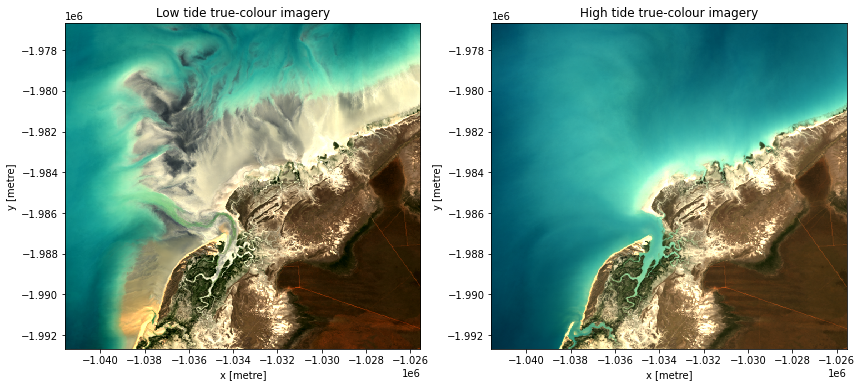
We can plot the data using the rgb function to view the loaded low and high tide imagery. By plotting the ['red', 'green', 'blue'] bands, we can view the imagery in true colour:

[7]:

# Plot low and high tide imagery side-by-side
fig, axes = plt.subplots(ncols=2, figsize=(14, 6))
rgb(low_tide_ds, bands=['red', 'green', 'blue'], ax=axes[0])
rgb(high_tide_ds, bands=['red', 'green', 'blue'], ax=axes[1])
axes[0].title.set_text('Low tide true-colour imagery')
axes[1].title.set_text('High tide true-colour imagery')

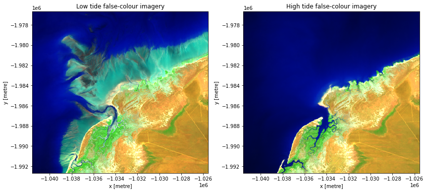
../../../_images/notebooks_DEA_products_DEA_High_and_Low_Tide_Imagery_17_0.png

By plotting the ['swir1', 'nir', 'green'] bands, we can view the imagery in false colour. This view emphasises the changing position of the land-water boundary between low and high tide.

Note: For more information about plotting satellite imagery in true and false colour, refer to the Introduction to Plotting notebook.

[8]:

# Plot low and high tide imagery side-by-side
fig, axes = plt.subplots(ncols=2, figsize=(14, 6))
rgb(low_tide_ds, bands=['swir1', 'nir', 'green'], ax=axes[0])
rgb(high_tide_ds, bands=['swir1', 'nir', 'green'], ax=axes[1])
axes[0].title.set_text('Low tide false-colour imagery')
axes[1].title.set_text('High tide false-colour imagery')

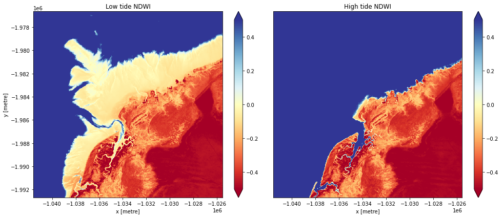
../../../_images/notebooks_DEA_products_DEA_High_and_Low_Tide_Imagery_19_0.png

Example application: computing remote sensing indices on low and high tide imagery

Because the DEA High and Low Tide Imagery data was produced using a geomedian approach that preserves the band relationships within the modelled spectra at each pixel, the surface reflectance values can be used for remote sensing applications (for example, image classification, remote sensing index calculation, habitat mapping) in exactly the same way as spectral bands from individual Landsat observations.

For example, we can use the data to compute simple remote sensing indices such as the Normalized Difference Water Index (NDWI). This index will have high values where a pixel is likely to be open water (e.g. NDWI > 0, or blue colours below):

[9]:

# Compute NDWI using the formula (green - nir) / (green + nir)
high_tide_ndwi = (high_tide_ds.green - high_tide_ds.nir) / \
                 (high_tide_ds.green + high_tide_ds.nir)
low_tide_ndwi = (low_tide_ds.green - low_tide_ds.nir) / \
                (low_tide_ds.green + low_tide_ds.nir)

# Plot high and low tide NDWI side-by-side
fig, axes = plt.subplots(ncols=2, figsize=(14, 6))
low_tide_ndwi.plot(ax=axes[0], vmin=-0.5, vmax=0.5, cmap='RdYlBu')
high_tide_ndwi.plot(ax=axes[1], vmin=-0.5, vmax=0.5, cmap='RdYlBu')
axes[0].title.set_text('Low tide NDWI')
axes[1].title.set_text('High tide NDWI')
axes[1].get_yaxis().set_visible(False)
fig.tight_layout()

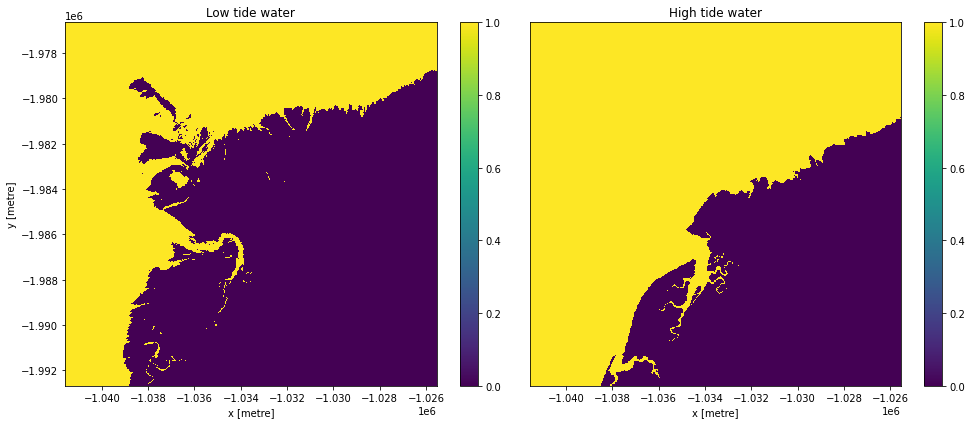
../../../_images/notebooks_DEA_products_DEA_High_and_Low_Tide_Imagery_21_0.png

A possible application of this may be to map the distribution of water at low and high tide using a NDWI threshold:

[10]:

# Identify water pixels using an example threshold value of 0
high_tide_water = high_tide_ndwi > 0
low_tide_water = low_tide_ndwi > 0

# Plot distribution of water at high and low tide
fig, axes = plt.subplots(ncols=2, figsize=(14, 6))
low_tide_water.plot(ax=axes[0])
high_tide_water.plot(ax=axes[1])
axes[0].title.set_text('Low tide water')
axes[1].title.set_text('High tide water')
axes[1].get_yaxis().set_visible(False)
fig.tight_layout()

../../../_images/notebooks_DEA_products_DEA_High_and_Low_Tide_Imagery_23_0.png

Additional information

License: The code in this notebook is licensed under the Apache License, Version 2.0. Digital Earth Australia data is licensed under the Creative Commons by Attribution 4.0 license.

Contact: If you need assistance, please post a question on the Open Data Cube Slack channel or on the GIS Stack Exchange using the open-data-cube tag (you can view previously asked questions here). If you would like to report an issue with this notebook, you can file one on GitHub.

Last modified: December 2023

Compatible datacube version:

[12]:

print(datacube.__version__)

1.8.5