Extracting contour lines 
Sign up to the DEA Sandbox to run this notebook interactively from a browser
Compatibility: Notebook currently compatible with both the
NCIandDEA SandboxenvironmentsProducts used: ga_srtm_dem1sv1_0
Background
Contour extraction is a fundamental image processing method used to detect and extract the boundaries of spatial features. While contour extraction has traditionally been used to precisely map lines of given elevation from digital elevation models (DEMs), contours can also be extracted from any other array-based data source. This can be used to support remote sensing applications where the position of a precise boundary needs to be mapped consistently over time, such as extracting dynamic waterline boundaries from satellite-derived remote sensing water index data (e.g. NDWI, MNDWI).
Description
This notebook demonstrates how to use the subpixel_contours function based on tools from skimage.measure.find_contours to:
Extract one or multiple contour lines from a single two-dimensional digital elevation model (DEM) and export these as a shapefile
Optionally include custom attributes in the extracted contour features
Load in a multi-dimensional satellite dataset from Digital Earth Australia, and extract a single contour value consistently through time along a specified dimension
Filter the resulting contours to remove small noisy features
Getting started
To run this analysis, run all the cells in the notebook, starting with the “Load packages” cell.
Load packages
[5]:
import sys
import datacube
import rioxarray
import numpy as np
import pandas as pd
import xarray as xr
import matplotlib as mpl
import matplotlib.pyplot as plt
from affine import Affine
from datacube.utils.geometry import CRS

import sys
sys.path.insert(1, '../Tools/')
from dea_tools.datahandling import load_ard
from dea_tools.bandindices import calculate_indices
from dea_tools.spatial import subpixel_contours
Connect to the datacube
[6]:
dc = datacube.Datacube(app='Contour_extraction')
Load elevation data
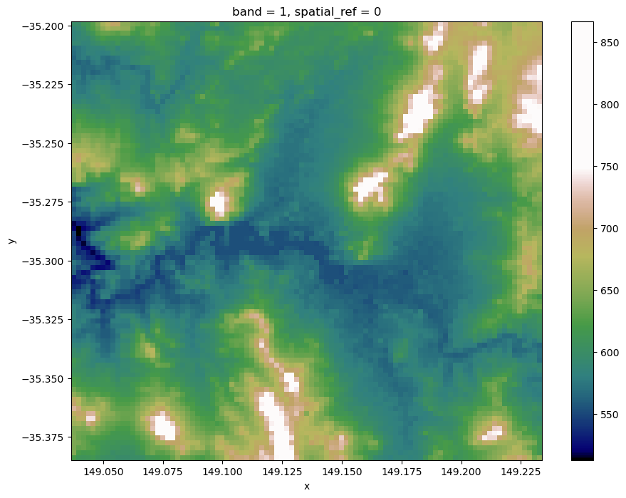
To demonstrate contour extraction, we first need to obtain an elevation dataset. Here we load a 250 m resolution Digital Elevation Model raster from the Shuttle Radar Topography Mission for the Canberra region (Jarvis et al. 2008) using the rioxarray.open_rasterio function.
[7]:
# Read in the elevation data from file
raster_path = '../Supplementary_data/Reprojecting_data/canberra_dem_250m.tif'
elevation_array = rioxarray.open_rasterio(raster_path).squeeze('band')

# Print the data
elevation_array
[7]:
<xarray.DataArray (y: 90, x: 95)>
[8550 values with dtype=int16]
Coordinates:
    band         int64 1
  * x            (x) float64 149.0 149.0 149.0 149.0 ... 149.2 149.2 149.2 149.2
  * y            (y) float64 -35.2 -35.2 -35.2 -35.21 ... -35.38 -35.38 -35.38
    spatial_ref  int64 0
Attributes:
    AREA_OR_POINT:  Area
    _FillValue:     -32768
    scale_factor:   1.0
add_offset: 0.0We can plot the elevation data using a custom terrain-coloured colour map:
[8]:
# Create a custom colourmap for the DEM
colors_terrain = plt.cm.gist_earth(np.linspace(0.0, 1.5, 100))
cmap_terrain = mpl.colors.LinearSegmentedColormap.from_list('terrain',
                                                            colors_terrain)

# Plot elevation data
elevation_array.plot(size=8, cmap=cmap_terrain)
[8]:
<matplotlib.collections.QuadMesh at 0x7fb0aaacde50>
Contour extraction in ‘single array, multiple z-values’ mode
The dea_spatialtools.subpixel_contours function uses skimage.measure.find_contours to extract contour lines from an array. This can be an elevation dataset like the data imported above, or any other two-dimensional or multi-dimensional array. We can extract contours from the elevation array imported above by providing a single z-value (e.g. elevation) or a list of z-values.
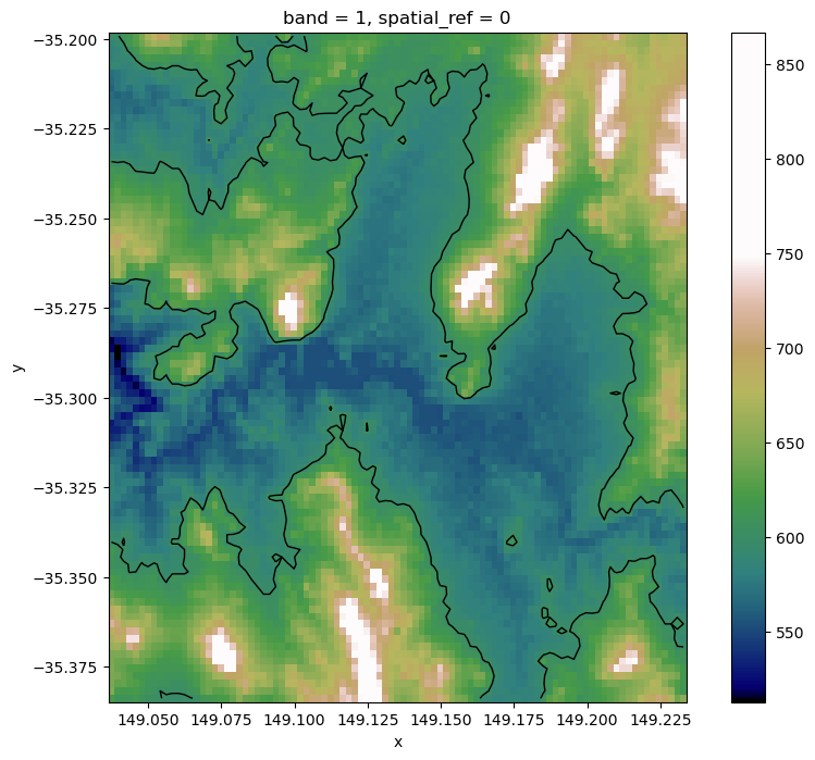
Extracting a single contour
Here, we extract a single 600 m elevation contour:
[9]:
# Extract contours
contours_gdf = subpixel_contours(da=elevation_array,
                                 z_values=600)

# Print output
contours_gdf
Operating in multiple z-value, single array mode
[9]:
| z_value | geometry | |
|---|---|---|
| 0 | 600 | MULTILINESTRING ((149.08043 -35.19917, 149.080... |
This returns a geopandas.GeoDataFrame containing a single contour line feature with the z-value (i.e. elevation) given in a shapefile field named z_value. We can plot contour this for the Canberra subset:
[10]:
elevation_array.plot(size=8, cmap=cmap_terrain)
contours_gdf.plot(ax=plt.gca(), linewidth=1.0, color='black')
[10]:
<Axes: title={'center': 'band = 1, spatial_ref = 0'}, xlabel='x', ylabel='y'>
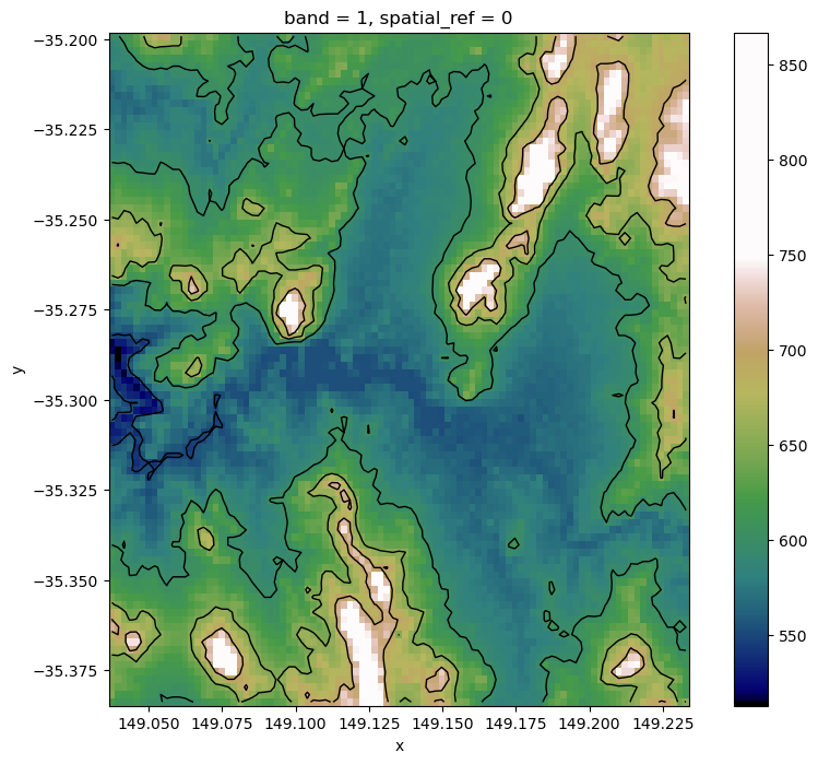
Extracting multiple contours
We can easily import multiple contours from a single array by supplying a list of z-values to extract. The function will then extract a contour for each value in z_values, skipping any contour elevation that is not found in the array.
[11]:
# List of elevations to extract
z_values = [500, 550, 600, 650, 700]

# Extract contours
contours_gdf = subpixel_contours(da=elevation_array,
                                 z_values=z_values)

# Plot extracted contours over the DEM
elevation_array.plot(size=8, cmap=cmap_terrain)
contours_gdf.plot(ax=plt.gca(), linewidth=1.0, color='black')
Operating in multiple z-value, single array mode
Failed to generate contours: 500
[11]:
<Axes: title={'center': 'band = 1, spatial_ref = 0'}, xlabel='x', ylabel='y'>
Custom shapefile attributes
By default, the shapefile includes a single z_value attribute field with one feature per input value in z_values. We can instead pass custom attributes to the output shapefile using the attribute_df parameter. For example, we might want a custom column called elev_cm with heights in cm instead of m, and a location column giving the location (Australian Capital Territory or ACT).
We can achieve this by first creating a pandas.DataFrame with column names giving the name of the attribute we want included with our contour features, and one row of values for each number in z_values:
[12]:
# Elevation values to extract
z_values = [550, 600, 650]

# Set up attribute dataframe (one row per elevation value above)
attribute_df = pd.DataFrame({'elev_cm': [55000, 60000, 65000],
                             'location': ['ACT', 'ACT', 'ACT']})

# Print output
attribute_df.head()
[12]:
| elev_cm | location | |
|---|---|---|
| 0 | 55000 | ACT |
| 1 | 60000 | ACT |
| 2 | 65000 | ACT |
We can now extract contours, and the resulting contour features will include the attributes we created above:
[13]:
# Extract contours with custom attribute fields:
contours_gdf = subpixel_contours(da=elevation_array,
                                 z_values=z_values,
                                 attribute_df=attribute_df)

# Print output
contours_gdf.head()
Operating in multiple z-value, single array mode
[13]:
| z_value | elev_cm | location | geometry | |
|---|---|---|---|---|
| 0 | 550 | 55000 | ACT | MULTILINESTRING ((149.03757 -35.31275, 149.039... |
| 1 | 600 | 60000 | ACT | MULTILINESTRING ((149.08043 -35.19917, 149.080... |
| 2 | 650 | 65000 | ACT | MULTILINESTRING ((149.06117 -35.19917, 149.061... |
Exporting contours to file
To export the resulting contours to file, use the output_path parameter. The function supports two output file formats:
GeoJSON (.geojson)
Shapefile (.shp)
[14]:
subpixel_contours(da=elevation_array,
                  z_values=z_values,
                  output_path='output_contours.geojson')
Operating in multiple z-value, single array mode
Writing contours to output_contours.geojson
[14]:
| z_value | geometry | |
|---|---|---|
| 0 | 550 | MULTILINESTRING ((149.03757 -35.31275, 149.039... |
| 1 | 600 | MULTILINESTRING ((149.08043 -35.19917, 149.080... |
| 2 | 650 | MULTILINESTRING ((149.06117 -35.19917, 149.061... |
Contours from non-elevation datasets in in ‘single z-value, multiple arrays’ mode
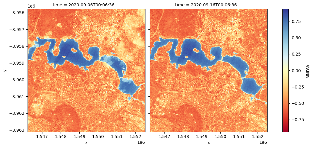
As well as extracting multiple contours from a single two-dimensional array, subpixel_contours also allows you to extract a single z-value from every array along a specified dimension in a multi-dimensional array. This can be useful for comparing the changes in the landscape across time. The input multi-dimensional array does not need to be elevation data: contours can be extracted from any type of data.
For example, we can use the function to extract the boundary between land and water (for a more in-depth analysis using contour extraction to monitor coastal erosion, see this notebook). First, we will load in a time series of Sentinel-2 imagery and calculate a simple Modified Normalized Difference Water Index (MNDWI) on two images. This index will have high values where a pixel is likely to be open water (e.g. MNDWI > 0, coloured in blue below):
[15]:
# Set up a datacube query to load data for
query = {'lat': (-35.27, -35.33),
         'lon': (149.09, 149.15),
         'time': ('2020-09-06', '2020-09-16'),
         'measurements': ['nbart_green', 'nbart_swir_2'],
         'output_crs': 'EPSG:3577',
         'resolution': (-20, 20)}

# Load Sentinel 2 data
s2_ds = dc.load(product='ga_s2am_ard_3',
                group_by='solar_day',
                **query)

# Calculate NDWI on the first and last image in the dataset
s2_ds = calculate_indices(s2_ds,
                          index='MNDWI',
                          collection='ga_s2_3')

# Plot the two images side by size
s2_ds.MNDWI.plot(col='time', cmap='RdYlBu', size=5)
[15]:
<xarray.plot.facetgrid.FacetGrid at 0x7fb0aa73ab20>
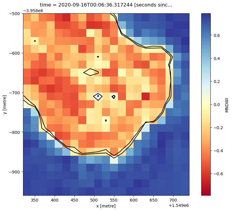
We can now identify the land-water boundary by extracting the 0 MNDWI contour for each array in the dataset along the time dimension. By plotting the resulting contour lines for a zoomed in area, we can then start to compare phenomenon like lake levels across time.
[16]:
# Extract the 0 MNDWI contour from both timesteps in the MNDWI data
contours_s2_gdf = subpixel_contours(da=s2_ds.MNDWI, z_values=0, dim='time')

# Plot contours over the top of array
s2_ds.MNDWI.sel(time='2020-09-16',
                x=slice(1549320, 1549733),
                y=slice(-3958494, -3958963)).plot(size=8, cmap='RdYlBu')
contours_s2_gdf.plot(ax=plt.gca(), linewidth=1.5, color='black');
Operating in single z-value, multiple arrays mode
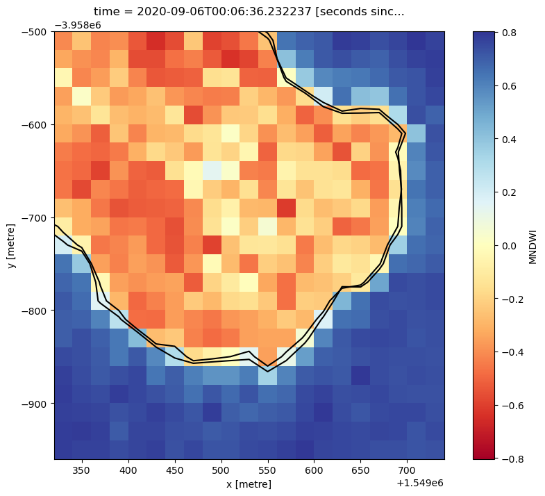
Dropping small contours
Contours produced by subpixel_contours can include many small features. We can optionally choose to extract only contours larger than a certain number of vertices using the min_vertices parameter. This can be useful for focusing on large contours, and remove possible noise in a dataset. Here we set min_vertices=10 to keep only contours with at least 10 vertices. Observe the tiny waterbodies in the middle of the image disappear:
[17]:
# Extract the 0 NDWI contour from both timesteps in the MNDWI data
contours_s2_gdf = subpixel_contours(da=s2_ds.MNDWI, z_values=0, min_vertices=10)

# Plot contours over the top of array
s2_ds.MNDWI.sel(time='2020-09-06',
                x=slice(1549320, 1549733),
                y=slice(-3958494, -3958963)).plot(size=8, cmap='RdYlBu')
contours_s2_gdf.plot(ax=plt.gca(), linewidth=1.5, color='black');
Operating in single z-value, multiple arrays mode
Exporting vector contours
To export our output contour data as a vector file (e.g. ESRI Shapefile or GeoJSON), just provide an output_path.
Here we export our data as a GeoJSON file called output.geojson:
[18]:
subpixel_contours(da=s2_ds.MNDWI,
                  z_values=0,
                  dim='time',
                  output_path='output.geojson')
Operating in single z-value, multiple arrays mode
Writing contours to output.geojson
[18]:
| time | geometry | |
|---|---|---|
| 0 | 2020-09-06 | MULTILINESTRING ((1549452.587 -3955790.000, 15... |
| 1 | 2020-09-16 | MULTILINESTRING ((1549451.796 -3955790.000, 15... |
Additional information
License: The code in this notebook is licensed under the Apache License, Version 2.0. Digital Earth Australia data is licensed under the Creative Commons by Attribution 4.0 license.
Contact: If you need assistance, please post a question on the Open Data Cube Slack channel or on the GIS Stack Exchange using the open-data-cube tag (you can view previously asked questions here). If you would like to report an issue with this notebook, you can file one on
GitHub.
Last modified: December 2023
Compatible datacube version:
[19]:
print(datacube.__version__)
1.8.13
Tags
Tags: NCI compatible, sandbox compatible, sentinel 2, load_ard, calculate_indices, subpixel_contours, contour extraction, image processing, MNDWI, downloading data, digital elevation model