Introduction to DEA Surface Reflectance (Landsat, Collection 3)

• Sign up to the DEA Sandbox to run this notebook interactively from a browser

• Compatibility: Notebook currently compatible with both the NCI and DEA Sandbox environments

• Products used: ga_ls8c_ard_3

Background

The United States Geological Survey’s (USGS) Landsat satellite program has been capturing images of the Australian continent for more than 30 years. These data are highly useful for land and coastal mapping studies. In particular, the light reflected from the Earth’s surface (surface reflectance) is important for monitoring environmental resources (such as agricultural production and mining activities) over time. We need to make accurate comparisons of imagery acquired at different times, seasons and geographic locations. However, inconsistencies can arise due to variations in atmospheric conditions, sun position, sensor view angle, surface slope and surface aspect. These inconsistencies need to be reduced or removed to ensure the data are consistent and can be compared over time.

What this product offers

DEA’s Landsat Surface Reflectance products take Landsat 5 Thematic Mapper (TM), Landsat 7 Enhanced Thematic Mapper Plus (ETM+) and Landsat 8 and 9 Operational Land Imager (OLI) imagery captured over the Australian continent and corrects for inconsistencies across land and coastal fringes. The result is accurate and standardised surface reflectance data, which is instrumental in identifying and quantifying environmental change.

DEA’s Landsat Surface Reflectance products form a single, cohesive Analysis Ready Data (ARD) package, which allows you to analyse surface reflectance data as is without the need to apply additional corrections.

It contains three sub-products that provide corrections or attribution information:

• Surface Reflectance NBAR (Landsat 5 TM, Landsat 7 ETM+, Landsat 8 OLI-TIRS, Landsat 9 OLI-TIRS)

• Surface Reflectance NBART (Landsat 5 TM, Landsat 7 ETM+, Landsat 8 OLI-TIRS, Landsat 9 OLI-TIRS)

• Surface Reflectance Observation Attributes (OA) (Landsat 5 TM, Landsat 7 ETM+, Landsat 8 OLI-TIRS, Landsat 9 OLI-TIRS)

The resolution is a 30 m grid based on the USGS Landsat Collection 1 archive.

Applications

• The development of derivative products to monitor land, inland waterways and coastal features, such as:

  • urban growth

  • coastal habitats

  • mining activities

  • agricultural activity (e.g. pastoral, irrigated cropping, rain-fed cropping)

  • water extent

• The development of refined information products, such as:

  • areal units of detected surface water

  • areal units of deforestation

  • yield predictions of agricultural parcels

• Compliance surveys

• Emergency management

Publications

• Li, F., Jupp, D. L. B., Reddy, S., Lymburner, L., Mueller, N., Tan, P., & Islam, A. (2010). An evaluation of the use of atmospheric and BRDF correction to standardize Landsat data. IEEE Journal of Selected Topics in Applied Earth Observations and Remote Sensing, 3(3), 257–270. https://doi.org/10.1109/JSTARS.2010.2042281

• Li, F., Jupp, D. L. B., Thankappan, M., Lymburner, L., Mueller, N., Lewis, A., & Held, A. (2012). A physics-based atmospheric and BRDF correction for Landsat data over mountainous terrain. Remote Sensing of Environment, 124, 756–770. https://doi.org/10.1016/j.rse.2012.06.018

Note: For more technical information about the DEA Landsat Surface Reflectance products, visit the official Geoscience Australia DEA Landsat Surface Reflectance product listings.

Description

This notebook will demonstrate how to load data from the DEA Landsat Surface Reflectance products using the Digital Earth Australia datacube. Topics covered include:

1. Inspecting the Landsat products and measurements available in the datacube

2. Loading Landsat data for a specific location and time

3. Plotting Landsat data in true and false colour

4. Applying a cloud mask using the ``oa_fmask` band <#Cloud-masking-using-the-Fmask-cloud-mask>`__

5. Advanced: Loading Landsat data in its native projection and resolution

6. Advanced: Filtering Landsat data by product metadata

---

Getting started

To run this analysis, run all the cells in the notebook, starting with the “Load packages” cell.

Load packages

Import Python packages that are used for the analysis.

import datacube
import matplotlib.pyplot as plt
from datacube.utils import masking

import sys
sys.path.insert(1, '../Tools/')
from dea_tools.datahandling import mostcommon_crs
from dea_tools.plotting import rgb
from dea_tools.datahandling import load_ard

Connect to the datacube

Connect to the datacube so we can access DEA data.

dc = datacube.Datacube(app='DEA_Landsat_Surface_Reflectance')

Available products and measurements

List products

We can use datacube’s list_products functionality to inspect the DEA Landsat Surface Reflectance products that are available in the datacube. The table below shows the product names that we will use to load the data, a brief description of the data, and the satellite instrument that acquired the data.

# List DEA Landsat Surface Reflectance products available in DEA
dc_products = dc.list_products()
dc_products.loc[['ga_ls5t_ard_3', 'ga_ls7e_ard_3', 'ga_ls8c_ard_3', 'ga_ls9c_ard_3']]

	name	description	license	default_crs	default_resolution
name
ga_ls5t_ard_3	ga_ls5t_ard_3	Geoscience Australia Landsat 5 Thematic Mapper...	CC-BY-4.0	None	None
ga_ls7e_ard_3	ga_ls7e_ard_3	Geoscience Australia Landsat 7 Enhanced Themat...	CC-BY-4.0	None	None
ga_ls8c_ard_3	ga_ls8c_ard_3	Geoscience Australia Landsat 8 Operational Lan...	CC-BY-4.0	None	None
ga_ls9c_ard_3	ga_ls9c_ard_3	Geoscience Australia Landsat 9 Operational Lan...	CC-BY-4.0	None	None

List measurements

We can further inspect the data available for each DEA Landsat Surface Reflectance product using datacube’s list_measurements functionality. The table below lists each of the measurements available in the data which have prefixes nbart_, nbar_ and oa_ that represent three main “sub-products” that provide corrections or attribution information for each Landsat product.

dc_measurements = dc.list_measurements()
dc_measurements.loc[['ga_ls8c_ard_3']]

		name	dtype	units	nodata	aliases	flags_definition
product	measurement
ga_ls8c_ard_3	nbart_coastal_aerosol	nbart_coastal_aerosol	int16	1	-999	[nbart_band01, coastal_aerosol]	NaN
	nbart_blue	nbart_blue	int16	1	-999	[nbart_band02, blue]	NaN
	nbart_green	nbart_green	int16	1	-999	[nbart_band03, green]	NaN
	nbart_red	nbart_red	int16	1	-999	[nbart_band04, red]	NaN
	nbart_nir	nbart_nir	int16	1	-999	[nbart_band05, nir, nbart_common_nir]	NaN
	nbart_swir_1	nbart_swir_1	int16	1	-999	[nbart_band06, swir_1, nbart_common_swir_1, sw...	NaN
	nbart_swir_2	nbart_swir_2	int16	1	-999	[nbart_band07, swir_2, nbart_common_swir_2, sw...	NaN
	nbart_panchromatic	nbart_panchromatic	int16	1	-999	[nbart_band08, panchromatic]	NaN
	oa_fmask	oa_fmask	uint8	1	0	[fmask]	{'fmask': {'bits': [0, 1, 2, 3, 4, 5, 6, 7], '...
	oa_nbart_contiguity	oa_nbart_contiguity	uint8	1	255	[nbart_contiguity]	{'contiguous': {'bits': [0], 'values': {'0': F...
	oa_azimuthal_exiting	oa_azimuthal_exiting	float32	1	NaN	[azimuthal_exiting]	NaN
	oa_azimuthal_incident	oa_azimuthal_incident	float32	1	NaN	[azimuthal_incident]	NaN
	oa_combined_terrain_shadow	oa_combined_terrain_shadow	uint8	1	255	[combined_terrain_shadow]	NaN
	oa_exiting_angle	oa_exiting_angle	float32	1	NaN	[exiting_angle]	NaN
	oa_incident_angle	oa_incident_angle	float32	1	NaN	[incident_angle]	NaN
	oa_relative_azimuth	oa_relative_azimuth	float32	1	NaN	[relative_azimuth]	NaN
	oa_relative_slope	oa_relative_slope	float32	1	NaN	[relative_slope]	NaN
	oa_satellite_azimuth	oa_satellite_azimuth	float32	1	NaN	[satellite_azimuth]	NaN
	oa_satellite_view	oa_satellite_view	float32	1	NaN	[satellite_view]	NaN
	oa_solar_azimuth	oa_solar_azimuth	float32	1	NaN	[solar_azimuth]	NaN
	oa_solar_zenith	oa_solar_zenith	float32	1	NaN	[solar_zenith]	NaN
	oa_time_delta	oa_time_delta	float32	1	NaN	[time_delta]	NaN

Surface Reflectance NBAR

Radiance data collected by Landsat 8 OLI-TIRS sensors can be affected by atmospheric conditions, sun position, sensor view angle, surface slope and surface aspect. These need to be reduced or removed to ensure the data can be compared consistently over time and space to identify and quantify environmental change. NBAR data (i.e. measurements with the nbar_ prefix above) takes Landsat imagery captured over the Australian continent and corrects the inconsistencies across land and coastal fringes using Nadir corrected Bi-directional reflectance distribution function Adjusted Reflectance (NBAR).

Note: NBAR data is currently only available in the NCI environment, not the DEA Sandbox.

Surface Reflectance NBART (with terrain illumination correction)

NBART data (i.e. measurements with the nbart_ prefix above) are also processed using NBAR, but have an additional terrain illumination correction applied using a Digital Surface Model (DSM) to correct for varying terrain (see Figure 1). NBART is typically the default choice for most analyses as removing terrain illumination and shadows allows changes in the landscape to be compared more consistently across time.

Figure 1: The animation above demonstrates how the NBART correction results in a significantly more two-dimensional looking image that is less affected by terrain illumination and shadow. Black pixels in the NBART image represent areas of deep terrain shadow that can’t be corrected as they’re determined not to be viewable by either the sun or the satellite. These are represented by -999 nodata values in the data. For more details about the difference between NBAR and NBART data, refer to the Introduction to Digital Earth Australia notebook, and the official DEA Landsat Surface Reflectance product listings.

Surface Reflectance Observation Attributes (OA)

The surface reflectance data produced by NBAR and NBART require accurate and reliable data provenance and information about the satellite data’s origins, derivations, methodology and processes. This allows the data to be reproducible and can increase the reliability of derivative applications. Attribution labels such as the location of cloud and cloud shadow pixels can be used to mask out these particular features from the surface reflectance analysis, or used as training data for machine learning algorithms. DEA’s Landsat surface reflectance data provides this information as “Observation Attribute” measurements with the prefix oa_. In the following Cloud masking section, we will demonstrate how to use OA data to create clear, cloud-free Landsat imagery.

The table produced by .list_measurements() also contains important information about the data type, nodata values and aliases available for each measurement contained in the product. Aliases (e.g. blue) can be used instead of the official measurement name (e.g. nbart_blue) when loading data (see next step).

Loading data

Now that we know what products and measurements are available for the products, we can load data from the datacube using dc.load.

In the example below, we will load data from Landsat 8 for Canberra from July 2021. We will load data from six spectral satellite bands, as well as cloud masking data ('oa_fmask'). By specifying output_crs='EPSG:3577' and resolution=(-30, 30), we request that datacube reproject our data to the Australian Albers coordinate reference system (CRS), with 30 x 30 m pixels. Finally, group_by='solar_day' ensures that overlapping images taken within seconds of each other as the satellite passes over are combined into a single time step in the data.

Note: For a more general discussion of how to load data using the datacube, refer to the Introduction to loading data notebook.

ls8_ds = dc.load(product='ga_ls8c_ard_3',
                 measurements=[
                     'nbart_red', 'nbart_green', 'nbart_blue', 'nbart_nir',
                     'nbart_swir_1', 'nbart_swir_2', 'oa_fmask'
                 ],
                 x=(149.05, 149.17),
                 y=(-35.25, -35.32),
                 time='2021-06-27',
                 group_by='solar_day')

We can now view the data that we loaded. The satellite bands listed under Data variables should match the measurements we requested above.

ls8_ds

<xarray.Dataset>
Dimensions:       (time: 1, y: 307, x: 395)
Coordinates:
  * time          (time) datetime64[ns] 2021-06-27T23:50:11.111104
  * y             (y) float64 -3.953e+06 -3.953e+06 ... -3.962e+06 -3.962e+06
  * x             (x) float64 1.543e+06 1.543e+06 ... 1.555e+06 1.555e+06
    spatial_ref   int32 3577
Data variables:
    nbart_red     (time, y, x) int16 563 679 593 539 532 ... 1323 1340 1267 1163
    nbart_green   (time, y, x) int16 602 657 622 494 527 ... 1217 1204 1163 1100
    nbart_blue    (time, y, x) int16 557 590 560 502 482 ... 1093 1091 1028 997
    nbart_nir     (time, y, x) int16 1370 1556 1603 1454 ... 1694 1648 1553 1568
    nbart_swir_1  (time, y, x) int16 907 993 1044 860 ... 1654 1545 1529 1476
    nbart_swir_2  (time, y, x) int16 633 734 671 534 519 ... 1500 1491 1396 1295
    oa_fmask      (time, y, x) uint8 1 1 1 1 1 1 1 1 1 1 ... 1 1 2 2 2 2 2 2 1 1
Attributes:
    crs:           EPSG:3577
    grid_mapping:  spatial_ref

xarray.Dataset

• Dimensions:
  • time: 1
  • y: 307
  • x: 395
• Coordinates: (4)
  • time
    (time)
    datetime64[ns]
    2021-06-27T23:50:11.111104

    units :

    seconds since 1970-01-01 00:00:00

    array(['2021-06-27T23:50:11.111104000'], dtype='datetime64[ns]')

  • y
    (y)
    float64
    -3.953e+06 ... -3.962e+06

    units :

    metre

    resolution :

    -30.0

    crs :

    EPSG:3577

    array([-3953085., -3953115., -3953145., ..., -3962205., -3962235., -3962265.])

  • x
    (x)
    float64
    1.543e+06 1.543e+06 ... 1.555e+06

    units :

    metre

    resolution :

    30.0

    crs :

    EPSG:3577

    array([1542795., 1542825., 1542855., ..., 1554555., 1554585., 1554615.])

  • spatial_ref
    ()
    int32
    3577

    spatial_ref :

    PROJCS["GDA94 / Australian Albers",GEOGCS["GDA94",DATUM["Geocentric_Datum_of_Australia_1994",SPHEROID["GRS 1980",6378137,298.257222101,AUTHORITY["EPSG","7019"]],AUTHORITY["EPSG","6283"]],PRIMEM["Greenwich",0,AUTHORITY["EPSG","8901"]],UNIT["degree",0.0174532925199433,AUTHORITY["EPSG","9122"]],AUTHORITY["EPSG","4283"]],PROJECTION["Albers_Conic_Equal_Area"],PARAMETER["latitude_of_center",0],PARAMETER["longitude_of_center",132],PARAMETER["standard_parallel_1",-18],PARAMETER["standard_parallel_2",-36],PARAMETER["false_easting",0],PARAMETER["false_northing",0],UNIT["metre",1,AUTHORITY["EPSG","9001"]],AXIS["Easting",EAST],AXIS["Northing",NORTH],AUTHORITY["EPSG","3577"]]

    grid_mapping_name :

    albers_conical_equal_area

    array(3577, dtype=int32)

• Data variables: (7)
  • nbart_red
    (time, y, x)
    int16
    563 679 593 539 ... 1340 1267 1163

    units :

    1

    nodata :

    -999

    crs :

    EPSG:3577

    grid_mapping :

    spatial_ref

    array([[[ 563,  679,  593, ...,  926, 1033,  923],
            [ 647,  523,  542, ..., 1050, 1317, 1201],
            [ 543,  502,  528, ..., 1022, 1191, 1040],
            ...,
            [7089, 7172, 7423, ..., 1196,  929, 1086],
            [5997, 6142, 6340, ..., 1362, 1263, 1171],
            [5221, 5218, 5504, ..., 1340, 1267, 1163]]], dtype=int16)

  • nbart_green
    (time, y, x)
    int16
    602 657 622 494 ... 1204 1163 1100

    units :

    1

    nodata :

    -999

    crs :

    EPSG:3577

    grid_mapping :

    spatial_ref

    array([[[ 602,  657,  622, ...,  931, 1021,  913],
            [ 572,  502,  486, ...,  954, 1279, 1042],
            [ 532,  523,  567, ...,  974, 1077, 1025],
            ...,
            [6761, 6824, 7056, ..., 1194,  986, 1095],
            [5692, 5835, 6073, ..., 1242, 1136, 1072],
            [5052, 5079, 5283, ..., 1204, 1163, 1100]]], dtype=int16)

  • nbart_blue
    (time, y, x)
    int16
    557 590 560 502 ... 1091 1028 997

    units :

    1

    nodata :

    -999

    crs :

    EPSG:3577

    grid_mapping :

    spatial_ref

    array([[[ 557,  590,  560, ...,  753,  809,  741],
            [ 560,  478,  508, ...,  812,  966,  833],
            [ 529,  488,  485, ...,  828,  953,  859],
            ...,
            [6462, 6517, 6719, ..., 1136,  901,  928],
            [5595, 5703, 5905, ..., 1126, 1017,  990],
            [4879, 4899, 5108, ..., 1091, 1028,  997]]], dtype=int16)

  • nbart_nir
    (time, y, x)
    int16
    1370 1556 1603 ... 1648 1553 1568

    units :

    1

    nodata :

    -999

    crs :

    EPSG:3577

    grid_mapping :

    spatial_ref

    array([[[1370, 1556, 1603, ..., 3738, 3665, 2900],
            [1499, 1799, 1781, ..., 3274, 4024, 3536],
            [1467, 1704, 2082, ..., 3285, 3274, 2937],
            ...,
            [7109, 7235, 7497, ..., 1948, 1954, 2600],
            [6111, 6229, 6498, ..., 1654, 1525, 1630],
            [5399, 5494, 5683, ..., 1648, 1553, 1568]]], dtype=int16)

  • nbart_swir_1
    (time, y, x)
    int16
    907 993 1044 860 ... 1545 1529 1476

    units :

    1

    nodata :

    -999

    crs :

    EPSG:3577

    grid_mapping :

    spatial_ref

    array([[[ 907,  993, 1044, ..., 2009, 2224, 1925],
            [1018,  911,  926, ..., 2243, 2798, 2341],
            [ 828,  887,  926, ..., 2122, 2328, 2142],
            ...,
            [5953, 6114, 6477, ..., 1707, 1474, 1976],
            [4910, 5104, 5402, ..., 1623, 1480, 1425],
            [4321, 4354, 4602, ..., 1545, 1529, 1476]]], dtype=int16)

  • nbart_swir_2
    (time, y, x)
    int16
    633 734 671 534 ... 1491 1396 1295

    units :

    1

    nodata :

    -999

    crs :

    EPSG:3577

    grid_mapping :

    spatial_ref

    array([[[ 633,  734,  671, ..., 1208, 1385, 1257],
            [ 706,  565,  576, ..., 1415, 1788, 1626],
            [ 561,  506,  523, ..., 1460, 1529, 1330],
            ...,
            [4851, 5065, 5450, ..., 1520, 1149, 1398],
            [3982, 4175, 4489, ..., 1561, 1355, 1302],
            [3344, 3424, 3704, ..., 1491, 1396, 1295]]], dtype=int16)

  • oa_fmask
    (time, y, x)
    uint8
    1 1 1 1 1 1 1 1 ... 2 2 2 2 2 2 1 1

    units :

    1

    nodata :

    0

    flags_definition :

    {'fmask': {'bits': [0, 1, 2, 3, 4, 5, 6, 7], 'values': {'0': 'nodata', '1': 'valid', '2': 'cloud', '3': 'shadow', '4': 'snow', '5': 'water'}, 'description': 'Fmask'}}

    crs :

    EPSG:3577

    grid_mapping :

    spatial_ref

    array([[[1, 1, 1, ..., 1, 1, 1],
            [1, 1, 1, ..., 1, 1, 1],
            [1, 1, 1, ..., 1, 1, 1],
            ...,
            [2, 2, 2, ..., 1, 1, 1],
            [2, 2, 2, ..., 2, 1, 1],
            [2, 2, 2, ..., 2, 1, 1]]], dtype=uint8)

• Indexes: (3)
  • time
    PandasIndex

    PandasIndex(DatetimeIndex(['2021-06-27 23:50:11.111104'], dtype='datetime64[ns]', name='time', freq=None))

  • y
    PandasIndex

    PandasIndex(Float64Index([-3953085.0, -3953115.0, -3953145.0, -3953175.0, -3953205.0,
                  -3953235.0, -3953265.0, -3953295.0, -3953325.0, -3953355.0,
                  ...
                  -3961995.0, -3962025.0, -3962055.0, -3962085.0, -3962115.0,
                  -3962145.0, -3962175.0, -3962205.0, -3962235.0, -3962265.0],
                 dtype='float64', name='y', length=307))

  • x
    PandasIndex

    PandasIndex(Float64Index([1542795.0, 1542825.0, 1542855.0, 1542885.0, 1542915.0, 1542945.0,
                  1542975.0, 1543005.0, 1543035.0, 1543065.0,
                  ...
                  1554345.0, 1554375.0, 1554405.0, 1554435.0, 1554465.0, 1554495.0,
                  1554525.0, 1554555.0, 1554585.0, 1554615.0],
                 dtype='float64', name='x', length=395))

• Attributes: (2)

  crs :

  EPSG:3577

  grid_mapping :

  spatial_ref

Plotting Landsat data

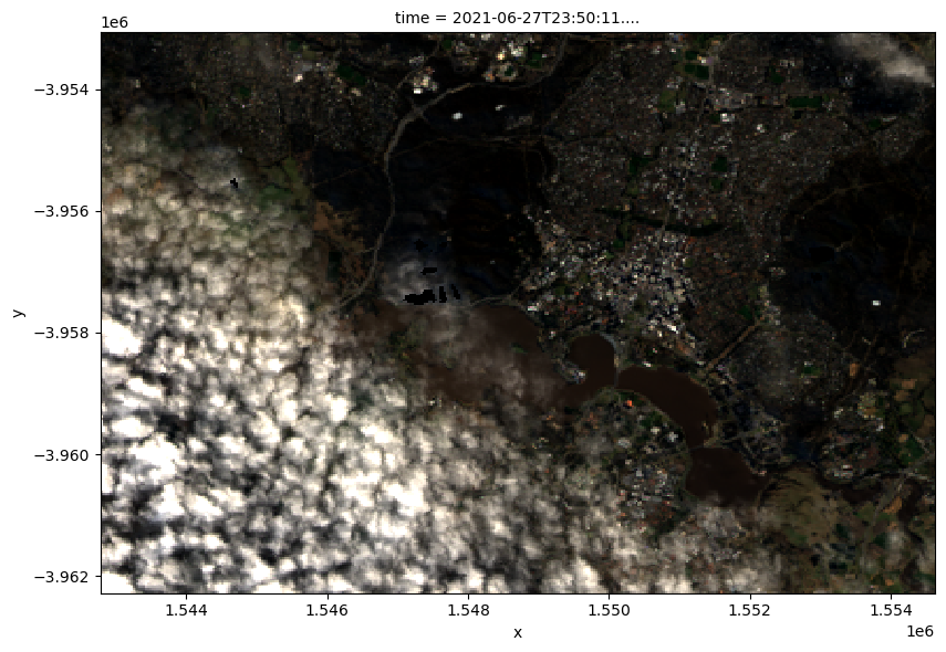
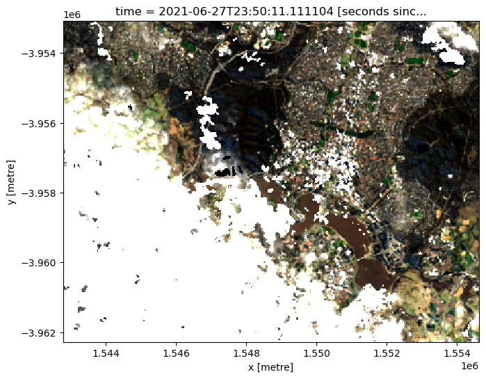
We can plot the data we loaded using the rgb function. By default, the function will plot data as a true colour image using the 'nbart_red', 'nbart_green', 'nbart_blue' bands.

rgb(ls8_ds, col='time')

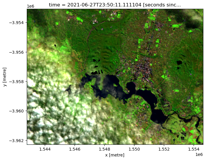
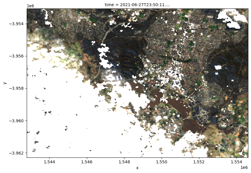
By plotting the ['nbart_swir_1', 'nbart_nir', 'nbart_green'] bands, we can view the imagery in false colour. This view emphasises growing vegetation in green and water in deep blue or black.

Note: For more information about plotting satellite imagery in true and false colour, refer to the Introduction to Plotting notebook.

rgb(ls8_ds, bands=['nbart_swir_1', 'nbart_nir', 'nbart_green'])

Cloud masking using the Fmask cloud mask

Many analyses might want to exclude targets that are obscured by cloud or cloud shadow. DEA Landsat Surface Reflectance data contains information about whether each pixel is likely to be free of clouds or shadow using an OA measurement band called oa_fmask. This band is calculated using the Fmask (Function of Mask) algorithm that classifies pixels using the following mutually exclusive numerical flags:

# Display available oa_fmask flags
masking.describe_variable_flags(ls8_ds.oa_fmask)['values'][0]

{'0': 'nodata',
 '1': 'valid',
 '2': 'cloud',
 '3': 'shadow',
 '4': 'snow',
 '5': 'water'}

ls8_ds.oa_fmask.plot()

<matplotlib.collections.QuadMesh at 0x7f56c49326a0>

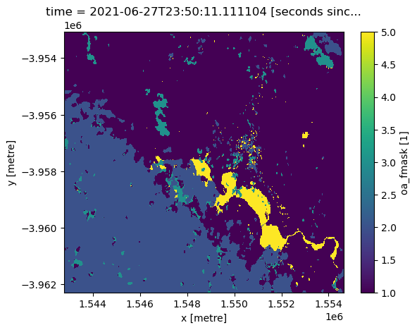
Of the six oa_fmask flags, 1 (clear), 4 (snow) and 5 (water) represent clear pixels that are not obscured by either cloud or cloud shadow. We can use these to create a mask that can be applied to other Landsat data to remove clouds or shadows before the data is analysed.

Note: Fmask’s “water” mask should typically not be relied to accurately analyse water using satellite data. Instead, consider loading data from the DEA Water Observations product instead.

# Identify pixels that are either "valid", "water" or "snow"
cloud_free_mask = (masking.make_mask(ls8_ds.oa_fmask, fmask="valid") |
                   masking.make_mask(ls8_ds.oa_fmask, fmask="water") |
                   masking.make_mask(ls8_ds.oa_fmask, fmask="snow"))

# Apply the mask
ls8_masked = ls8_ds.where(cloud_free_mask)

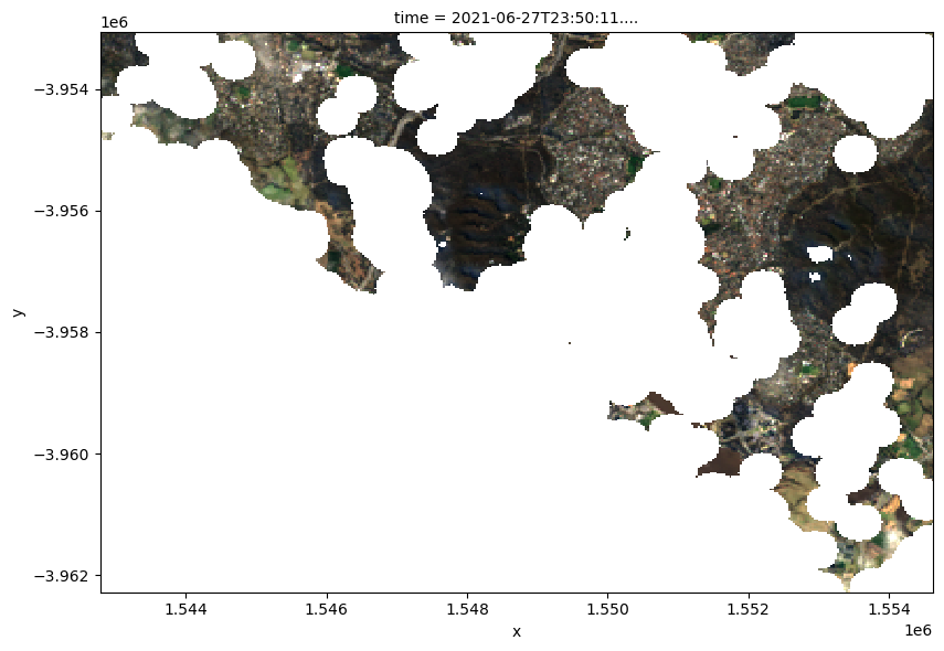
If we plot our masked data, we can see that the areas of cloud and cloud shadow above have now been masked out (i.e. area of NaN values or white pixels):

rgb(ls8_masked)

/env/lib/python3.8/site-packages/matplotlib/cm.py:478: RuntimeWarning: invalid value encountered in cast
  xx = (xx * 255).astype(np.uint8)

Limitations of Fmask for cloud masking Landsat data

Fmask has limitations due to the complex nature of detecting natural phenomena such as cloud. For example, bright targets such as beaches, buildings and salt lakes often get mistaken for clouds. Edges and fringes of clouds also tend to be more transparent and can be missed by the cloud detection algorithm.

Because of these limitations, it can be advisable to treat individual FMask classifications with caution, and use analysis techniques that are robust to any potential classification errors (e.g. temporal median or geomedian composites that will supress the effect of false positive or negative cloud classifications).

Note: For more information about Fmask and other Surface Reflectance Observation Attributes, refer to the Observation Attributes product description listings for Landsat 5, 7 and 8. For a more detailed guide to masking satellite data (and dealing with common issues such as false positive cloud detection, refer to the Masking data notebook.

Loading cloud-masked Landsat with load_ard

Another option for loading Landsat data is the load_ard() function, which is a wrapper function around the dc.load() function. Compared to dc.load, this function allows you to load multiple Landsat satellite sensors at once, and automatically filter and mask by cloud. The result is an analysis-ready dataset.

In the example below, we show how to load the same Landsat 8 image using load_ard, automatically applying a cloud mask to the data.

Note: Find more information about load_ard in the detailed Using load ard notebook.

ds_ard = load_ard(dc=dc,
                  products=['ga_ls8c_ard_3'],
                  measurements=[
                      'nbart_red',
                      'nbart_green',
                      'nbart_blue',
                  ],
                  x=(149.05, 149.17),
                  y=(-35.25, -35.32),
                  time='2021-06-27',
                  group_by='solar_day')

rgb(ds_ard, col='time', vmin=0, vmax=2000)

Finding datasets
    ga_ls8c_ard_3
Applying fmask pixel quality/cloud mask
Loading 1 time steps

/env/lib/python3.8/site-packages/matplotlib/cm.py:478: RuntimeWarning: invalid value encountered in cast
  xx = (xx * 255).astype(np.uint8)

The function supports an additional mask_filters parameter that allows you to apply dilation around the clouds in your cloud mask. For example, here we can pass mask_filters=[("dilation", 10)] to dilate our clouds by 10 pixels on every side, ensuring that thin cloud edges are correctly masked out:

ds_ard = load_ard(dc=dc,
                  products=['ga_ls8c_ard_3'],
                  measurements=[
                      'nbart_red',
                      'nbart_green',
                      'nbart_blue',
                  ],
                  x=(149.05, 149.17),
                  y=(-35.25, -35.32),
                  time='2021-06-27',
                  group_by='solar_day',
                  mask_filters=[("dilation", 10)])

rgb(ds_ard, col='time', vmin=0, vmax=2000)

Finding datasets
    ga_ls8c_ard_3
Applying morphological filters to pixel quality mask: [('dilation', 10)]
Applying fmask pixel quality/cloud mask
Loading 1 time steps

/home/jovyan/Tools/dea_tools/datahandling.py:492: UserWarning: As of `dea_tools` v0.3.0, pixel quality masks are inverted before being passed to `mask_filters` (i.e. so that good quality/clear pixels are False and poor quality pixels/clouds are True). This means that 'dilation' will now expand cloudy pixels, rather than shrink them as in previous versions.
  warnings.warn(
/env/lib/python3.8/site-packages/rasterio/warp.py:344: NotGeoreferencedWarning: Dataset has no geotransform, gcps, or rpcs. The identity matrix will be returned.
  _reproject(

Note: For a more detailed guide to cloud masking satellite data (and dealing with common issues such as false positive cloud detection, refer to the Masking data notebook.

Advanced

Native load

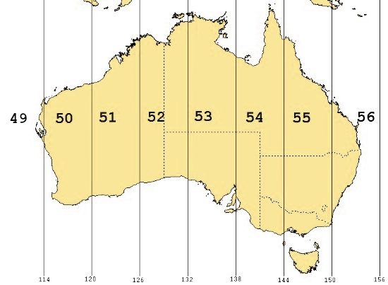
DEA Landsat Surface Reflectance data is originally processed from USGS Collection 1 data which is stored on file in different Universal Transverse Mercator (UTM) CRSs depending on the longitude of the data. There are 8 UTM zones (and therefore unique Landsat CRSs) that cover Australia:

Reprojecting these data into a single projection system like Australian Albers (EPSG:3577) will force datacube to resample the data to fit this new spatial grid. This can lead to artefacts in the resulting imagery that can affect its usefulness for precise applications (e.g. using Landsat to accurately map the boundary between land and water using sub-pixel techniques).

Determining native projection and spatial resolution

Because of this, it can be useful to load Landsat data in its “native” projection and spatial resolution — that is, load the data into the same spatial grid as it is stored on file without applying any reprojection or resampling. To achieve this, we need to first determine which of the UTM zones above apply for a given location, and use this information to load our data into that CRS. We can do this using DEA’s mostcommon_crs function which takes a datacube query, then identifies the most common CRS for all data that matches the query without having to load this data into memory first.

First, we will set up a query covering the same time and location previously used to load data:

query = {
    'x': (149.05, 149.17),
    'y': (-35.25, -35.32),
    'time': '2021-06-27',
}

We can now pass this to mostcommon_crs. In this example, the most common CRS is 'epsg:32655' or UTM Zone 55 (this matches the map above).

# Determine the most common CRS for the query
native_crs = mostcommon_crs(dc, product='ga_ls8c_ard_3', query=query)
native_crs

'epsg:32655'

We can now pass this CRS to dc.load()’s output_crs parameter to load Landsat data in its native spatial grid. The native resolution of all DEA Landsat Surface Reflectance data (with the exception of Landsat 8’s panchromatic band; see the Pansharpening notebook) is 30 m, so we can supply this to resolution directly without having to obtain it from the data.

Using the align parameter when natively loading data

In addition to output_crs and resolution, one final parameter is required to construct the spatial grid used for natively loading Landsat data: align. By default, datacube assumes that pixel edges are aligned such that x=0 and y=0 lines fall on pixel edges. However, Landsat data is stored on file with coordinates that define the centre - not the edge - of each pixel. When natively loading data, to ensure the spatial pixel grid created by datacube is exactly the same grid as used by Landsat imagery, we need to shift this grid by 15 m in both directions by specifying align=(15, 15). Otherwise, natively loaded pixels will be offset by half a pixel from their true location.

To determine whether you need to use align when loading DEA Landsat Surface Reflectance data, all the following must apply:

• You are loading Landsat data from the ga_ls5t_ard_3, ga_ls7e_ard_3 and ga_ls8c_ard_3 products that define pixel coordinates by their centers rather than pixel edges

• You want to load data in its native projection without a half pixel offset

• You are supplying a native UTM zone CRS generated by mostcommon_crs or copied from a datacube dataset

• You are supplying a native resolution (e.g. resolution=(-30, 30))

Note: You should also use the align parameter when natively loading data from the DEA Water Observations and DEA Fractional Cover products.

# Load Landsat using native CRS, resolution and appropriate alignment
ls8_native = dc.load(product='ga_ls8c_ard_3',
                     measurements=['nbart_red', 'nbart_green', 'nbart_blue'],
                     output_crs=native_crs,
                     resolution=(-30, 30),
                     align=(15, 15),
                     group_by='solar_day',
                     **query)

Note: If a study area extends across the boundary of two UTM zones, it is possible that a single datacube query will return data with multiple CRSs. In this scenario, although mostcommon_crs will return the native CRS that will involve the least overall reprojection or resampling, some data will unavoidably need to be reprojected and resampled away from its native CRS and resolution. If this is the case, mostcommon_crs will print a warning to inform you that multiple CRSs were encounted for the query. To minimise the impacts of this reprojection, you can specify a resampling method that will only be used to transform the subset of satellite observations that do not match the CRS generated by mostcommon_crs (for more information about resampling, refer to the dc.load documentation).

Filtering by metadata

In addition to generic dc.load query parameters (e.g. product, measurements, time, x, y etc), DEA Landsat Surface Reflectance data contains a set of extra metadata fields that can be queried to filter data before it is loaded. Searchable metadata fields for a product can be listed using the code below:

dataset = dc.find_datasets(product='ga_ls8c_ard_3', limit=1)[0]
dir(dataset.metadata)

['cloud_cover',
 'creation_dt',
 'creation_time',
 'crs_raw',
 'dataset_maturity',
 'eo_gsd',
 'eo_sun_azimuth',
 'eo_sun_elevation',
 'fmask_clear',
 'fmask_cloud_shadow',
 'fmask_snow',
 'fmask_water',
 'format',
 'gqa',
 'gqa_abs_iterative_mean_x',
 'gqa_abs_iterative_mean_xy',
 'gqa_abs_iterative_mean_y',
 'gqa_abs_x',
 'gqa_abs_xy',
 'gqa_abs_y',
 'gqa_cep90',
 'gqa_iterative_mean_x',
 'gqa_iterative_mean_xy',
 'gqa_iterative_mean_y',
 'gqa_iterative_stddev_x',
 'gqa_iterative_stddev_xy',
 'gqa_iterative_stddev_y',
 'gqa_mean_x',
 'gqa_mean_xy',
 'gqa_mean_y',
 'gqa_stddev_x',
 'gqa_stddev_xy',
 'gqa_stddev_y',
 'grid_spatial',
 'id',
 'instrument',
 'label',
 'landsat_product_id',
 'landsat_scene_id',
 'lat',
 'lon',
 'measurements',
 'platform',
 'product_family',
 'region_code',
 'sources',
 'time']

Some of the most useful metadata fields for filtering Landsat data before loading it include:

• gqa_iterative_mean_xy: An estimate of how accurately a satellite scene is georeferenced, calculated by comparing hundreds of candidate Ground Control Points, then discarding outliers to obtain a more robust estimate. Values are in pixel units based on a 25 metre resolution reference image (i.e. 0.2 = 5 metres)

This parameter can be used to ensure that we only load data that is closely aligned spatially through time. For example, to load only imagery with a geometric accuracy of less than 12.5 m (e.g. 50% of the 25 m reference pixel), we can add gqa_iterative_mean_xy=(0, 0.5) to our dc.load query:

ls8_geo = dc.load(product='ga_ls8c_ard_3',
                  measurements=['nbart_red', 'nbart_green', 'nbart_blue'],
                  x=(149.05, 149.17),
                  y=(-35.25, -35.32),
                  time=('2021-06', '2021-09'),
                  gqa_iterative_mean_xy=(0, 0.5),
                  group_by='solar_day')

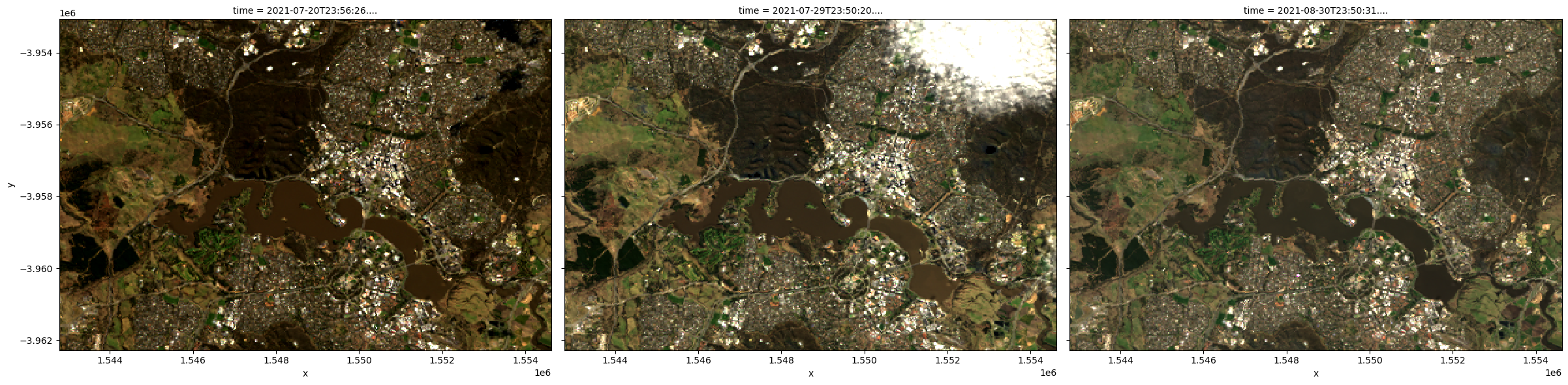
• cloud_cover: This gives an estimate of the percentage (i.e. from 0 to 100) of each satellite scene that contains cloud (as measured by Fmask).

For example, to filter imagery to data from scenes with between 0 and 5% cloud, we can add cloud_cover=(0, 5) to our dc.load query:

ls8_nocloud = dc.load(product='ga_ls8c_ard_3',
                      measurements=['nbart_red', 'nbart_green', 'nbart_blue'],
                      x=(149.05, 149.17),
                      y=(-35.25, -35.32),
                      time=('2021-06', '2021-09'),
                      cloud_cover=(0, 5),
                      group_by='solar_day')

# Plot imagery to verify they are mostly cloud-free
rgb(ls8_nocloud, col='time')

Note: Metadata provides a single value for each entire Landsat satellite scene, not the specific location specified by dc.load. For example, cloud_cover provides an estimate of cloudiness for each full Landsat scene that intersects with your query, which may not reflect the cloudiness of the smaller sub-region you have requested using x and y. For a more accurate method for filtering satellite data by the cloudiness of a specific study area, refer to the Filtering to non-cloudy observations section of the Using load_ard notebook.

---

Additional information

License: The code in this notebook is licensed under the Apache License, Version 2.0. Digital Earth Australia data is licensed under the Creative Commons by Attribution 4.0 license.

Contact: If you need assistance, please post a question on the Open Data Cube Slack channel or on the GIS Stack Exchange using the open-data-cube tag (you can view previously asked questions here). If you would like to report an issue with this notebook, you can file one on GitHub.

Last modified: December 2023

Compatible datacube version:

print(datacube.__version__)

1.8.13

Tags

Tags: NCI compatible, sandbox compatible, DEA products, landsat 5, landsat 7, landsat 8, landsat 9, rgb, mostcommon_crs, masking, cloud masking, native load, metadata