Introduction to DEA Mangroves

Sign up to the DEA Sandbox to run this notebook interactively from a browser
Compatibility: Notebook currently compatible with the DEA Sandbox environment
Products used: ga_ls_mangrove_cover_cyear_3

Background

Mangroves are unique, valuable and vulnerable woody plant species that inhabit intertidal regions around much of the Australian coastline.

They provide a diverse array of ecosystem services such as:

coastal protection
carbon storage
nursery grounds and habitat for a huge variety of avian, coastal and marine animal species.

However, mangrove ecosystems are impacted upon by both natural and anthropogenic drivers of change such as sea-level rise, coastal land reclaimation and severe tropical cyclone damage. In Australia, mangroves are protected by law and consequently, changes in their extent and canopy density are driven predominantly by natural drivers.

Modelling mangrove canopy density offers an effective mechanism to assess how mangroves are responding to these external influences and to monitor their recovery to ensure that they can continue to thrive and support our vital coastal ecosystems.

What this product offers

The DEA Mangroves data product maps the annual canopy cover density of Australian mangroves within a fixed extent around the entire continental coastline. The extent represents a union of Global Mangrove Watch layers for multiple years, produced by the Japanese Aerospace Exploration Agency.

Within this extent, mangroves are identified by leveraging a relationship between the 10th percentile green vegetation component of the DEA Fractional Cover data product with Light Detection And Ranging (LiDAR)-derived Planimetric Canopy Cover% (PCC). More detail on the method can be found here.

Three cover classes are identified within the product which are defined as:

Closed Forest - pixels with more than 80 % mangrove canopy cover
Open Forest - pixels with between 50 % and 80 % canopy cover
Woodland - pixels with between 20 % and 50 % canopy cover

Publications

Lymburner, L., Bunting, P., Lucas, R., Scarth, P., Alam, I., Phillips, C., Ticehurst, C., & Held, A., (2020). Mapping the multi-decadal mangrove dynamics of the Australian coastline. Remote Sensing of Environment, 238, 111185.

Description

This notebook introduces the DEA Mangroves data product and steps through how to:

View the product name and associated measurements in the DEA database
Load the dataset and view the data classes within it
Plot a single timestep image
Create and view an animation of the whole timeseries
Plot change over time by graphing the timeseries of each class
Identify hotspot change areas within each class

Getting started

To run this analysis, run all the cells in the notebook, starting with the “Load packages” cell.

Load packages

Import Python packages that are used for the analysis.

[1]:

%matplotlib inline

import datacube
import matplotlib.pyplot as plt
import numpy as np
import pandas as pd

from datacube.utils import masking
from IPython.core.display import Video
from matplotlib.colors import LinearSegmentedColormap

import sys

sys.path.insert(1, "../Tools/")
from dea_tools.plotting import display_map, xr_animation

Connect to the datacube

Connect to the datacube so we can access DEA data. The app parameter is a unique name for the analysis which is based on the notebook file name.

[2]:

dc = datacube.Datacube(app="DEA_Mangroves")

Available products and measurements

List products available in Digital Earth Australia

[3]:

dc_products = dc.list_products()
dc_products.loc[["ga_ls_mangrove_cover_cyear_3"]]

[3]:

	name	description	license	default_crs	default_resolution
name
ga_ls_mangrove_cover_cyear_3	ga_ls_mangrove_cover_cyear_3	Geoscience Australia Landsat Mangrove Cover Ca...	CC-BY-4.0	None	None

List measurements

View the list of measurements associated with the DEA Mangroves product. Note the single measurement unit, the nodata value and the flags_definitions.

[4]:

dc_measurements = dc.list_measurements()
dc_measurements.loc[["ga_ls_mangrove_cover_cyear_3"]]

[4]:

		name	dtype	units	nodata	aliases	flags_definition
product	measurement
ga_ls_mangrove_cover_cyear_3	canopy_cover_class	canopy_cover_class	uint8	1	255	NaN	{'woodland': {'bits': [0, 1, 2, 3, 4, 5, 6, 7]...

Loading data

Select and view your study area

If running the notebook for the first time, keep the default settings below. This will demonstrate how the analysis works and provide meaningful results. Zoom around the displayed map to understand the context of the analysis area. To select a new area, click on the map to reveal the Latitude (y) and Longitude (x) for diagonally opposite corners and place these values into the query

Replace the y and x coordinates to try the following locations:

Bowling Green Bay, Qld
- “y”: (-19.50688750115376, -19.27501266742088)
- “x”: (147.05183029174404, 147.47617721557216)
Pellew Islands, NT
- “y”: (-15.6786, -16.0075)
- “x”: (136.5360, 137.0682)

[5]:

# Set up a region to load data
query = {
    "y": (-15.6806, -15.8193),
    "x": (136.5202, 136.6885),
    "time": ("1988", "2022"),
}
display_map(x=query["x"], y=query["y"])

[5]:

Make this Notebook Trusted to load map: File -> Trust Notebook

View the DEA Mangroves class values and definitions

You’ll see that four classes are identified in this dataset. The notobserved class was separated from nodata pixels in this workflow to identify locations where mangroves have been observed but there is poor observation density. This class is usually insignificant in size and has not been included in the remainder of this notebook analysis.

[7]:

# Extract the flags information from the dataset
flags = masking.describe_variable_flags(mangroves)
flags["bits"] = flags["bits"].astype(str)
flags = flags.sort_values(by="bits")

# Append the class descriptions to each class
descriptors = {
    "closed_forest": "> 80 % canopy cover",
    "open_forest": "50 - 80 % canopy cover",
    "woodland": "20 - 50 % canopy cover",
    "notobserved": "Fewer than 3 clear observations",
}
flags = flags.rename(columns={"description": "class"})
flags["description"] = pd.Series(data=descriptors, index=flags.index)

# View the values in the dataset that are associated with each class
flags

[7]:

	bits	values	class	description
woodland	[0, 1, 2, 3, 4, 5, 6, 7]	{'1': True}	Woodland	20 - 50 % canopy cover
notobserved	[0, 1, 2, 3, 4, 5, 6, 7]	{'0': True}	Mangroves not observed	Fewer than 3 clear observations
open_forest	[0, 1, 2, 3, 4, 5, 6, 7]	{'2': True}	Open Forest	50 - 80 % canopy cover
closed_forest	[0, 1, 2, 3, 4, 5, 6, 7]	{'3': True}	Closed Forest	> 80 % canopy cover

Plotting data

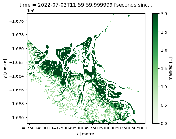
Plot a single timestep

[8]:

# Firstly, mask out the nodata values
mangroves["masked"] = mangroves.canopy_cover_class.where(mangroves.canopy_cover_class != 255)

# Plot the most recent timestep
mangroves["masked"].isel(time=-1).plot(cmap="Greens")

[8]:

<matplotlib.collections.QuadMesh at 0x7f25cde04100>

../../../_images/notebooks_DEA_products_DEA_Mangroves_22_1.png

View all timesteps as an animation

[9]:

# Produce a time series animation of mangrove canopy cover
xr_animation(
    ds=mangroves,
    bands=["masked"],
    output_path="DEA_Mangroves.mp4",
    annotation_kwargs={"fontsize": 20, "color": "white"},
    show_date="%Y",
    imshow_kwargs={"cmap": "Greens"},
    show_colorbar=True,
    interval=1000,
    width_pixels=800,
)

# Plot animation
plt.close()

# View and interact with the animation
Video("DEA_Mangroves.mp4", embed=True)

Exporting animation to DEA_Mangroves.mp4

[9]:

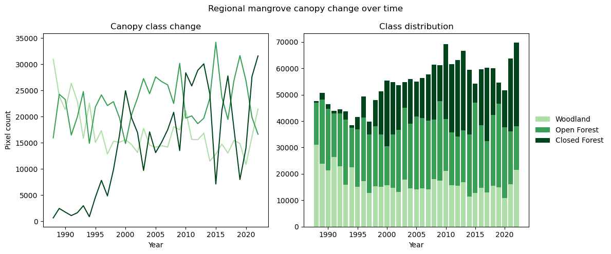
Plot the area (number of pixels) occupied by each class at every timestep in the area of interest

[10]:

# Set up the data for plotting: count the number of pixels per class in the loaded location
mangroves["closed_forest"]= mangroves.canopy_cover_class.where(mangroves.canopy_cover_class == 3)
mangroves["open_forest"] = mangroves.canopy_cover_class.where(mangroves.canopy_cover_class == 2)
mangroves["woodland"] = mangroves.canopy_cover_class.where(mangroves.canopy_cover_class == 1)

y1 = mangroves["woodland"].count(dim=["y", "x"])
y2 = mangroves["open_forest"].count(dim=["y", "x"])
y3 = mangroves["closed_forest"].count(dim=["y", "x"])

# Simplify the date labels for the x-axis
x = np.arange(int(query["time"][0]), int(query["time"][-1]) + 1, 1)

# Prepare the figures
fig, axs = plt.subplots(1, 2, figsize=(12, 5))
fig.suptitle("Regional mangrove canopy change over time")

# Plot the single class summaries
axs[0].plot(x, y1, color="#aedea7", label="Woodland")
axs[0].plot(x, y2, color="#37a055", label="Open Forest")
axs[0].plot(x, y3, color="#00441b", label="Closed Forest")
axs[0].set_title("Canopy class change")
axs[0].set(ylabel="Pixel count", xlabel="Year")

# Stack the classes to plot a snapshot of the region at each time step
axs[1].bar(x, y1, color="#aedea7", label="Woodland")
axs[1].bar(x, y2, color="#37a055", label="Open Forest", bottom=y1)
axs[1].bar(x, y3, color="#00441b", label="Closed Forest", bottom=(y1 + y2))
axs[1].legend(bbox_to_anchor=(1.0, 0.5), loc="center left", frameon=False)
axs[1].set_title("Class distribution")
axs[1].set(xlabel="Year")

plt.tight_layout()
plt.show()

../../../_images/notebooks_DEA_products_DEA_Mangroves_26_0.png

Example applications

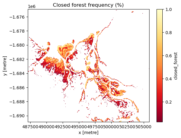
Detect change hotspots in each class

Identify change hotspots in the analysis area by assessing the frequency that each class was identified during the length of the timeseries.

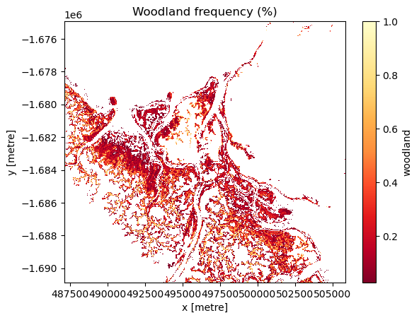
Pale yellow coloured areas signify pixels that have a high frequency of being identified as the class of interest over the length of the timeseries and were consistently modelled as that class. Orange to red areas are pixels that were less frequently identified as the class of interest during the timeseries and thus, experienced change between classes during the timeseries.

[11]:

# Create a boolean mask of the `Closed Forest` class
mangroves["closed_forest"] = masking.make_mask(mangroves.canopy_cover_class, closed_forest=True)
# Calculate the frequency of each pixel being identified as `Closed Forest` during the timeseries
mg_cf = mangroves["closed_forest"].mean(dim=["time"])
# Mask out values of 0 to ensure a clean visualisation
mg_cf.where(mg_cf > 0).plot(cmap='YlOrRd_r')
# Title the plot
plt.title("Closed forest frequency (%)")

[11]:

Text(0.5, 1.0, 'Closed forest frequency (%)')

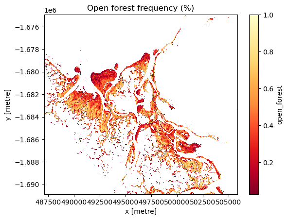
../../../_images/notebooks_DEA_products_DEA_Mangroves_28_1.png

[12]:

# Create a boolean mask of the `Open Forest' class
mangroves["open_forest"] = masking.make_mask(mangroves.canopy_cover_class, open_forest=True)
# Calculate the frequency of each pixel being identified as `Open Forest` during the timeseries
mg_of = mangroves["open_forest"].mean(dim=["time"])
# Mask out values of 0 to ensure a clean visualisation
mg_of.where(mg_of > 0).plot(cmap='YlOrRd_r')
# Title the plot
plt.title("Open forest frequency (%)")

[12]:

Text(0.5, 1.0, 'Open forest frequency (%)')

../../../_images/notebooks_DEA_products_DEA_Mangroves_29_1.png

[13]:

# Create a boolean mask of the `Woodland' class
mangroves["woodland"] = masking.make_mask(mangroves.canopy_cover_class, woodland=True)
# Calculate the frequency of each pixel being identified as `Woodland` during the timeseries
mg_wl = mangroves["woodland"].mean(dim=["time"])
# Mask out values of 0 to ensure a clean visualisation
mg_wl.where(mg_wl > 0).plot(cmap='YlOrRd_r')
# Title the plot
plt.title("Woodland frequency (%)")

[13]:

Text(0.5, 1.0, 'Woodland frequency (%)')

../../../_images/notebooks_DEA_products_DEA_Mangroves_30_1.png

Additional information

License: The code in this notebook is licensed under the Apache License, Version 2.0. Digital Earth Australia data is licensed under the Creative Commons by Attribution 4.0 license.

Contact: If you need assistance, please post a question on the Open Data Cube Slack channel or on the GIS Stack Exchange using the open-data-cube tag (you can view previously asked questions here). If you would like to report an issue with this notebook, you can file one on GitHub.

Last modified: December 2023

Compatible datacube version: 1.8.13

[14]:

print(datacube.__version__)

1.8.13