Polygon drill

• Sign up to the DEA Sandbox to run this notebook interactively from a browser

• Compatibility: Notebook currently compatible with both the NCI and DEA Sandbox environments

• Products used: ga_ls8c_ard_3

• Special requirements: A vector file (e.g. GeoJSON, Esri Shapefile) containing the polygon you would like to use for the analysis. Here we use a polygon extracted from the ACT Suburb/Locality Boundaries Administrative Boundaries © Geoscape Australia dataset.

Description

A polygon drill can be used to grab a stack of imagery that corresponds to the location of an input polygon. It is a useful tool for generating animations, or running analyses over long time periods.

This notebook shows you how to:

1. Use a polygon’s geometry to generate a dc.load query

2. Mask the returned data with the polygon geometry (to remove unwanted pixels)

3. Plot a timeseries plot summarising satellite bands over time

---

Getting started

To run this analysis, run all the cells in the notebook, starting with the “Load packages” cell.

Load packages

Import Python packages that are used for the analysis.

%matplotlib inline

import datacube
import geopandas as gpd
import odc.geo.xr
from odc.geo.geom import Geometry

import sys

sys.path.insert(1, "../Tools/")
from dea_tools.plotting import rgb

Connect to the datacube

Connect to the datacube so we can access DEA data. The app parameter is a unique name for the analysis which is based on the notebook file name.

dc = datacube.Datacube(app="Polygon_drill")

Analysis parameters

Update the following two parameters to set the polygon dataset and times used for the polygon drill:

• polygon_to_drill: The path containing the vector file to use for the polygon drill. If it’s a local file, then this parameter is the local path to that polygon. If it’s located online, then this is the path to the online location of the polygon.

• time_to_drill: e.g. ('2020-02', '2020-03'). The time over which we want to run the polygon drill, entered as a tuple.

For this example, we will use a polygon for Capital Hill in Canberra extracted from the ACT Suburb/Locality Boundaries Administrative Boundaries © Geoscape Australia vector dataset, licensed by the Commonwealth of Australia under Creative Commons Attribution 4.0 International licence (CC BY 4.0).

polygon_to_drill = (
    "../Supplementary_data/Polygon_drill/act_localities_capitalhill.geojson"
)
time_to_drill = ("2020-01", "2020-03")

Load the vector file we want to use for the polygon drill

# Read vector file
polygon_to_drill = gpd.read_file(polygon_to_drill)

# Check that the polygon loaded as expected. We'll just print the first 3 rows to check
polygon_to_drill.head(3)

	LC_PLY_PID	LOC_PID	DT_CREATE	LOC_NAME	LOC_CLASS	STATE	geometry
0	lcpb8f6c0999acd	loceae77f35464f	2022-03-11	Capital Hill	Gazetted Locality	ACT	MULTIPOLYGON (((149.12849 -35.31083, 149.12848...

Query the datacube using the polygon we have loaded

Set up the dc.load query

We need to grab the polygon from the vector file we want to use for the polygon drill. For this example, we’ll just grab the first polygon from the file using .iloc[0] (Capital Hill in the ACT).

To use this polygon in datacube, we need to first convert it to a odc.geo.geom.Geometry object. This is the equivelent of a shapely geometry, but with added Coordinate Reference System information (for more information, refer to the odc-geo documentation).

# Select polygon
shapely_geometry = polygon_to_drill.iloc[0].geometry

# Convert to Geometry object with CRS information
geom = Geometry(geom=shapely_geometry, crs=polygon_to_drill.crs)
geom

To set up the query, we need to set up several additional parameters:

• geopolygon: Here we input the geometry we want to use for the drill that we prepared in the cell above

• time: Feed in the time_to_drill parameter we set earlier

• output_crs: We need to specify the coordinate reference system (CRS) of the output. We’ll use Albers Equal Area projection for Australia

• resolution: You can choose the resolution of the output dataset. Since Landsat 8 is 30 m resolution, we’ll just use that

• measurements: Here is where you specify which bands you want to extract. We will just be plotting a true colour image, so we just need red, green and blue.

query = {
    "geopolygon": geom,
    "time": time_to_drill,
    "output_crs": "EPSG:3577",
    "resolution": (-30, 30),
    "measurements": ["nbart_red", "nbart_green", "nbart_blue"],
}

Use the query to extract data

Here we have chosen to load data from Landsat 8 by supplying product='ga_ls8c_ard_3', but this can be changed depending on your requirements.

We can verify that the polygon drill has loaded a time series of satellite data by checking the Dimensions of the resulting xarray.Dataset. In this example, we can see that the polygon drill has loaded 11 time steps (i.e. Dimensions: time: 11):

# Load data for our polygon and time period
ds = dc.load(product="ga_ls8c_ard_3", group_by="solar_day", **query)

# Check we have some data back with multiple timesteps
ds

<xarray.Dataset>
Dimensions:      (time: 11, y: 33, x: 32)
Coordinates:
  * time         (time) datetime64[ns] 2020-01-07T23:56:40.592891 ... 2020-03...
  * y            (y) float64 -3.96e+06 -3.96e+06 ... -3.961e+06 -3.961e+06
  * x            (x) float64 1.549e+06 1.549e+06 1.549e+06 ... 1.55e+06 1.55e+06
    spatial_ref  int32 3577
Data variables:
    nbart_red    (time, y, x) int16 1043 1157 1222 1061 ... 2403 2743 3157 3047
    nbart_green  (time, y, x) int16 1014 1116 1150 1023 ... 2321 2650 2972 2935
    nbart_blue   (time, y, x) int16 944 1019 1029 932 ... 2201 2491 2862 2848
Attributes:
    crs:           EPSG:3577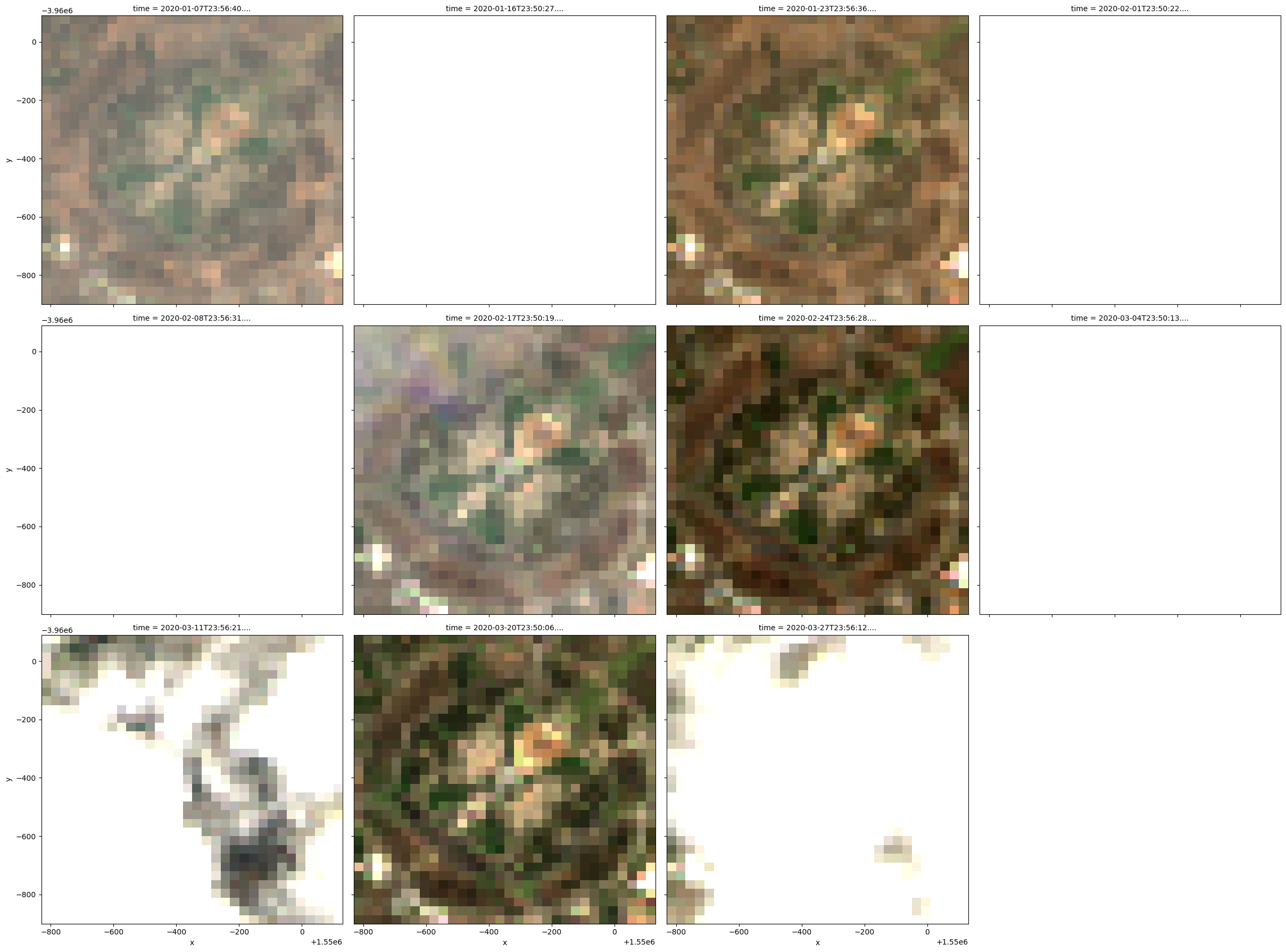
    grid_mapping:  spatial_ref

xarray.Dataset

• Dimensions:
  • time: 11
  • y: 33
  • x: 32
• Coordinates: (4)
  • time
    (time)
    datetime64[ns]
    2020-01-07T23:56:40.592891 ... 2...

    units :

    seconds since 1970-01-01 00:00:00

    array(['2020-01-07T23:56:40.592891000', '2020-01-16T23:50:27.927367000',
           '2020-01-23T23:56:36.765939000', '2020-02-01T23:50:22.661832000',
           '2020-02-08T23:56:31.774346000', '2020-02-17T23:50:19.161045000',
           '2020-02-24T23:56:28.025939000', '2020-03-04T23:50:13.948244000',
           '2020-03-11T23:56:21.709961000', '2020-03-20T23:50:06.289323000',
           '2020-03-27T23:56:12.950767000'], dtype='datetime64[ns]')

  • y
    (y)
    float64
    -3.96e+06 -3.96e+06 ... -3.961e+06

    units :

    metre

    resolution :

    -30.0

    crs :

    EPSG:3577

    array([-3959925., -3959955., -3959985., -3960015., -3960045., -3960075.,
           -3960105., -3960135., -3960165., -3960195., -3960225., -3960255.,
           -3960285., -3960315., -3960345., -3960375., -3960405., -3960435.,
           -3960465., -3960495., -3960525., -3960555., -3960585., -3960615.,
           -3960645., -3960675., -3960705., -3960735., -3960765., -3960795.,
           -3960825., -3960855., -3960885.])

  • x
    (x)
    float64
    1.549e+06 1.549e+06 ... 1.55e+06

    units :

    metre

    resolution :

    30.0

    crs :

    EPSG:3577

    array([1549185., 1549215., 1549245., 1549275., 1549305., 1549335., 1549365.,
           1549395., 1549425., 1549455., 1549485., 1549515., 1549545., 1549575.,
           1549605., 1549635., 1549665., 1549695., 1549725., 1549755., 1549785.,
           1549815., 1549845., 1549875., 1549905., 1549935., 1549965., 1549995.,
           1550025., 1550055., 1550085., 1550115.])

  • spatial_ref
    ()
    int32
    3577

    spatial_ref :

    PROJCS["GDA94 / Australian Albers",GEOGCS["GDA94",DATUM["Geocentric_Datum_of_Australia_1994",SPHEROID["GRS 1980",6378137,298.257222101,AUTHORITY["EPSG","7019"]],AUTHORITY["EPSG","6283"]],PRIMEM["Greenwich",0,AUTHORITY["EPSG","8901"]],UNIT["degree",0.0174532925199433,AUTHORITY["EPSG","9122"]],AUTHORITY["EPSG","4283"]],PROJECTION["Albers_Conic_Equal_Area"],PARAMETER["latitude_of_center",0],PARAMETER["longitude_of_center",132],PARAMETER["standard_parallel_1",-18],PARAMETER["standard_parallel_2",-36],PARAMETER["false_easting",0],PARAMETER["false_northing",0],UNIT["metre",1,AUTHORITY["EPSG","9001"]],AXIS["Easting",EAST],AXIS["Northing",NORTH],AUTHORITY["EPSG","3577"]]

    grid_mapping_name :

    albers_conical_equal_area

    array(3577, dtype=int32)

• Data variables: (3)
  • nbart_red
    (time, y, x)
    int16
    1043 1157 1222 ... 2743 3157 3047

    units :

    1

    nodata :

    -999

    crs :

    EPSG:3577

    grid_mapping :

    spatial_ref

    array([[[1043, 1157, 1222, ..., 1255, 1296, 1377],
            [1047, 1149, 1022, ..., 1332, 1309, 1333],
            [1150, 1037, 1043, ..., 1303, 1224, 1089],
            ...,
            [1292, 1268, 1275, ..., 1522, 1601, 1416],
            [1302, 1227, 1267, ..., 1413, 1549, 1545],
            [1250, 1226, 1177, ..., 1382, 1786, 1534]],
    
           [[4381, 4378, 4396, ..., 3929, 4091, 4375],
            [4209, 4386, 4432, ..., 4039, 4190, 4445],
            [4138, 4312, 4429, ..., 4214, 4355, 4487],
            ...,
            [3775, 3853, 3999, ..., 4468, 4293, 3850],
            [3383, 3407, 3647, ..., 4466, 4261, 3862],
            [3323, 3336, 3599, ..., 4276, 4096, 3703]],
    
           [[ 898, 1051, 1070, ..., 1087, 1052, 1110],
            [ 846,  969,  783, ..., 1028,  951,  932],
            [1019,  847,  827, ...,  918,  869,  900],
            ...,
    ...
            ...,
            [4176, 3532, 2820, ..., 2472, 2526, 2998],
            [4743, 4138, 2967, ..., 1984, 2077, 2497],
            [5568, 4772, 3484, ..., 1760, 1879, 2341]],
    
           [[ 570,  893,  987, ...,  771,  853, 1047],
            [ 558,  734,  687, ...,  797,  859,  869],
            [ 575,  626,  794, ...,  764,  685,  635],
            ...,
            [ 881,  913,  862, ..., 1304, 1521, 1029],
            [ 947,  928, 1007, ..., 1499, 1467, 1075],
            [ 753,  774,  742, ..., 1808, 1921, 1541]],
    
           [[1227, 1710, 1648, ..., 2063, 2256, 2454],
            [1727, 1700, 1339, ..., 1933, 2236, 2461],
            [1962, 1935, 1893, ..., 2262, 2595, 2714],
            ...,
            [1265, 1319, 1375, ..., 2853, 3062, 3274],
            [1520, 1442, 1486, ..., 2774, 3197, 3285],
            [1577, 1470, 1591, ..., 2743, 3157, 3047]]], dtype=int16)

  • nbart_green
    (time, y, x)
    int16
    1014 1116 1150 ... 2650 2972 2935

    units :

    1

    nodata :

    -999

    crs :

    EPSG:3577

    grid_mapping :

    spatial_ref

    array([[[1014, 1116, 1150, ..., 1149, 1216, 1278],
            [1011, 1098,  998, ..., 1202, 1229, 1246],
            [1069, 1034, 1052, ..., 1243, 1157, 1052],
            ...,
            [1213, 1184, 1162, ..., 1359, 1332, 1248],
            [1202, 1153, 1178, ..., 1300, 1416, 1380],
            [1184, 1132, 1095, ..., 1274, 1399, 1343]],
    
           [[4364, 4366, 4390, ..., 3984, 4189, 4438],
            [4211, 4358, 4415, ..., 4101, 4213, 4478],
            [4131, 4295, 4410, ..., 4284, 4405, 4545],
            ...,
            [3763, 3874, 3986, ..., 4456, 4291, 3880],
            [3468, 3453, 3674, ..., 4451, 4267, 3895],
            [3386, 3398, 3654, ..., 4278, 4108, 3733]],
    
           [[ 768,  893,  923, ...,  883,  939, 1015],
            [ 728,  878,  731, ...,  914,  937,  921],
            [ 797,  776,  788, ...,  933,  823,  763],
            ...,
    ...
            ...,
            [4004, 3362, 2784, ..., 2335, 2488, 2941],
            [4599, 3938, 2815, ..., 1935, 2018, 2381],
            [5284, 4601, 3364, ..., 1746, 1833, 2329]],
    
           [[ 580,  865,  989, ...,  766,  849, 1072],
            [ 569,  665,  662, ...,  790,  918,  926],
            [ 668,  637,  836, ...,  881,  743,  629],
            ...,
            [ 922,  862,  755, ..., 1090, 1057,  697],
            [ 872,  785,  825, ..., 1342, 1325, 1094],
            [ 691,  677,  655, ..., 1343, 1488, 1301]],
    
           [[1246, 1635, 1589, ..., 1973, 2169, 2364],
            [1723, 1670, 1322, ..., 1889, 2163, 2394],
            [1855, 1889, 1842, ..., 2206, 2500, 2590],
            ...,
            [1278, 1276, 1216, ..., 2682, 2914, 3158],
            [1393, 1273, 1308, ..., 2697, 3156, 3116],
            [1468, 1353, 1526, ..., 2650, 2972, 2935]]], dtype=int16)

  • nbart_blue
    (time, y, x)
    int16
    944 1019 1029 ... 2491 2862 2848

    units :

    1

    nodata :

    -999

    crs :

    EPSG:3577

    grid_mapping :

    spatial_ref

    array([[[ 944, 1019, 1029, ..., 1050, 1085, 1118],
            [ 945,  997,  950, ..., 1057, 1053, 1072],
            [ 982,  952,  973, ..., 1053, 1033,  982],
            ...,
            [1085, 1085, 1068, ..., 1190, 1188, 1155],
            [1101, 1074, 1070, ..., 1131, 1198, 1164],
            [1074, 1047, 1030, ..., 1145, 1243, 1176]],
    
           [[4413, 4400, 4370, ..., 4124, 4272, 4507],
            [4246, 4369, 4389, ..., 4196, 4368, 4613],
            [4171, 4351, 4425, ..., 4402, 4582, 4685],
            ...,
            [3927, 4016, 4116, ..., 4447, 4314, 3945],
            [3634, 3621, 3809, ..., 4464, 4298, 3950],
            [3495, 3509, 3729, ..., 4336, 4180, 3833]],
    
           [[ 539,  686,  697, ...,  649,  670,  728],
            [ 561,  681,  555, ...,  643,  605,  603],
            [ 571,  590,  616, ...,  583,  571,  573],
            ...,
    ...
            ...,
            [3791, 3258, 2677, ..., 2314, 2454, 2854],
            [4336, 3714, 2692, ..., 1864, 1934, 2292],
            [5001, 4363, 3235, ..., 1661, 1721, 2253]],
    
           [[ 440,  627,  735, ...,  522,  587,  703],
            [ 405,  563,  521, ...,  543,  548,  561],
            [ 433,  483,  595, ...,  496,  469,  442],
            ...,
            [ 675,  651,  546, ...,  818,  796,  615],
            [ 641,  606,  632, ...,  932,  926,  692],
            [ 505,  514,  478, ..., 1022, 1047,  982]],
    
           [[1008, 1375, 1386, ..., 1807, 2009, 2188],
            [1462, 1462, 1109, ..., 1708, 1972, 2222],
            [1648, 1625, 1616, ..., 2003, 2322, 2348],
            ...,
            [1044, 1019,  990, ..., 2568, 2764, 3044],
            [1116, 1055, 1061, ..., 2515, 2848, 2949],
            [1260, 1146, 1207, ..., 2491, 2862, 2848]]], dtype=int16)

• Indexes: (3)
  • time
    PandasIndex

    PandasIndex(DatetimeIndex(['2020-01-07 23:56:40.592891', '2020-01-16 23:50:27.927367',
                   '2020-01-23 23:56:36.765939', '2020-02-01 23:50:22.661832',
                   '2020-02-08 23:56:31.774346', '2020-02-17 23:50:19.161045',
                   '2020-02-24 23:56:28.025939', '2020-03-04 23:50:13.948244',
                   '2020-03-11 23:56:21.709961', '2020-03-20 23:50:06.289323',
                   '2020-03-27 23:56:12.950767'],
                  dtype='datetime64[ns]', name='time', freq=None))

  • y
    PandasIndex

    PandasIndex(Float64Index([-3959925.0, -3959955.0, -3959985.0, -3960015.0, -3960045.0,
                  -3960075.0, -3960105.0, -3960135.0, -3960165.0, -3960195.0,
                  -3960225.0, -3960255.0, -3960285.0, -3960315.0, -3960345.0,
                  -3960375.0, -3960405.0, -3960435.0, -3960465.0, -3960495.0,
                  -3960525.0, -3960555.0, -3960585.0, -3960615.0, -3960645.0,
                  -3960675.0, -3960705.0, -3960735.0, -3960765.0, -3960795.0,
                  -3960825.0, -3960855.0, -3960885.0],
                 dtype='float64', name='y'))

  • x
    PandasIndex

    PandasIndex(Float64Index([1549185.0, 1549215.0, 1549245.0, 1549275.0, 1549305.0, 1549335.0,
                  1549365.0, 1549395.0, 1549425.0, 1549455.0, 1549485.0, 1549515.0,
                  1549545.0, 1549575.0, 1549605.0, 1549635.0, 1549665.0, 1549695.0,
                  1549725.0, 1549755.0, 1549785.0, 1549815.0, 1549845.0, 1549875.0,
                  1549905.0, 1549935.0, 1549965.0, 1549995.0, 1550025.0, 1550055.0,
                  1550085.0, 1550115.0],
                 dtype='float64', name='x'))

• Attributes: (2)

  crs :

  EPSG:3577

  grid_mapping :

  spatial_ref

Plot original satellite data

To inspect the satellite data we have loaded using the pixel drill, we can plot an image for each timestep in the data:

rgb(ds, col="time", vmin=0, vmax=2000)

Mask data using polygon

The data returned from our polygon drill contains data for the bounding box (i.e. extents) of the input polygon, not the actual shape of the polygon. To get rid of the parts of the image located outside the polygon, we need to mask our using the original polygon.

This can be achieved easily using the built-in .odc.mask() method on our xarray data, which will set all pixels outside of the mask to nan to signify “nodata”:

# Mask out all pixels outside of our polygon:
ds_masked = ds.odc.mask(poly=geom)

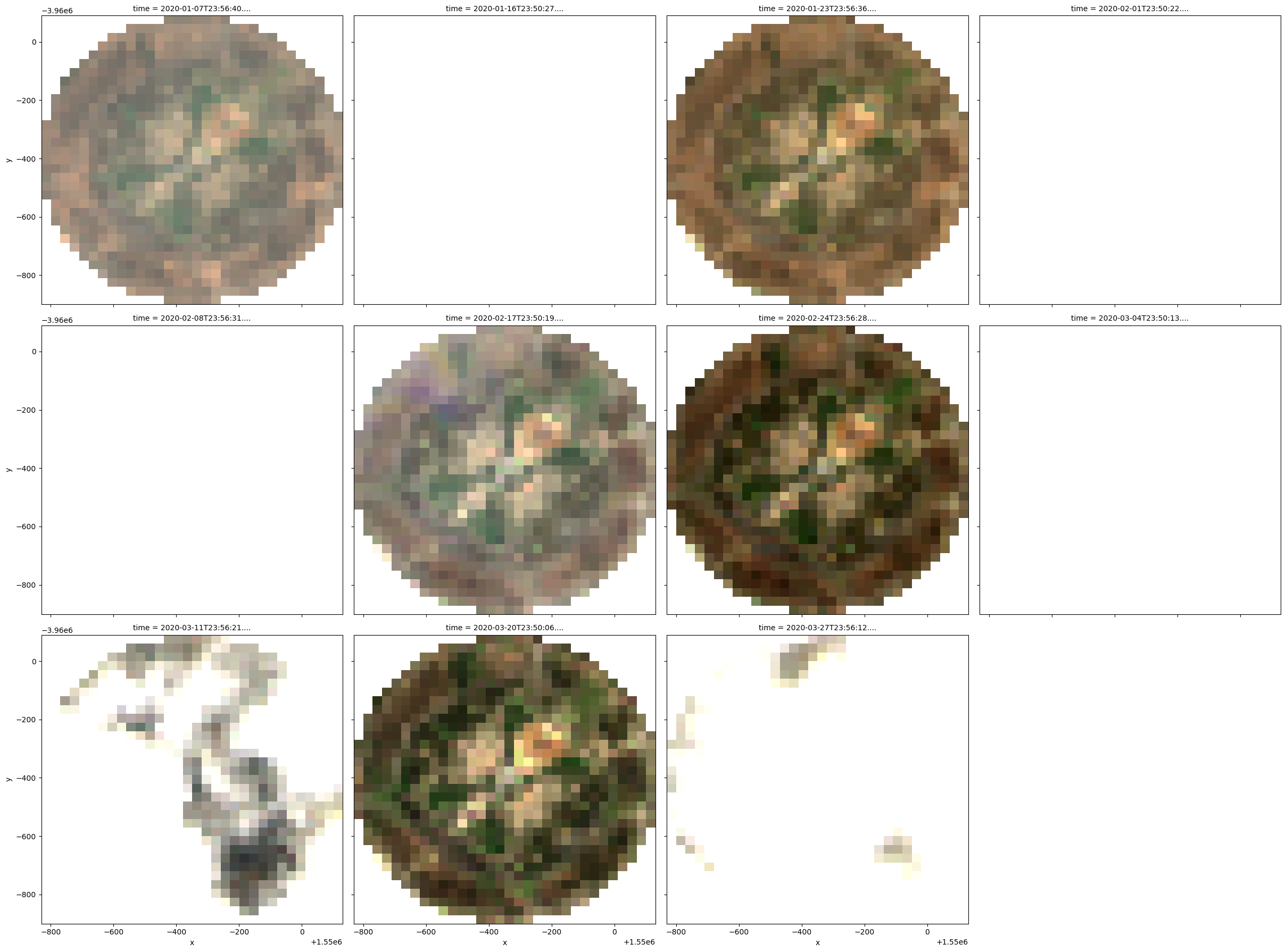
Plot masked data

When we plot this new masked dataset, we can see that the areas located outside of the polygon have now been masked out (i.e. set to nan or white).

Note: Several of our images are also covered in cloud - for advice on applying a cloud mask to remove these cloudy pixels see the Masking data using the Fmask cloud mask notebook.

rgb(ds_masked, col="time", vmin=0, vmax=2000)

/env/lib/python3.10/site-packages/matplotlib/cm.py:494: RuntimeWarning: invalid value encountered in cast
  xx = (xx * 255).astype(np.uint8)

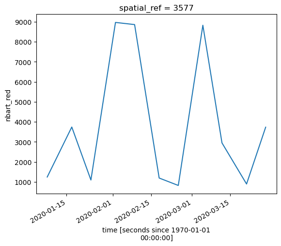
Summarise results over time into a timeseries plot

Now that we have produced a masked satellite dataset, we can summarise values across time to plot it as a polygon drill timeseries. This can be useful for summarising environmental change over time (e.g. drying or wetting of the landscape, or the growth or less of vegetation cover).

# Average of the red band across time
red_timeseries = ds_masked.nbart_red.mean(dim=["x", "y"])
red_timeseries.plot()

[<matplotlib.lines.Line2D at 0x7fae8e2351e0>]

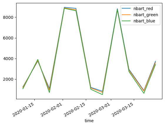
We can also summarise all of our bands across time as a pandas.Dataframe(), and plot them on a single graph:

# Plot all bands at once
timeseries_df = ds_masked.mean(dim=["x", "y"]).drop("spatial_ref").to_dataframe()
display(timeseries_df)
timeseries_df.plot()

	nbart_red	nbart_green	nbart_blue
time
2020-01-07 23:56:40.592891	1243.424683	1170.858887	1051.900391
2020-01-16 23:50:27.927367	3740.156494	3802.088867	3901.860107
2020-01-23 23:56:36.765939	1093.314331	936.836304	692.188599
2020-02-01 23:50:22.661832	8965.114258	8898.247070	8858.674805
2020-02-08 23:56:31.774346	8857.622070	8714.263672	8629.692383
2020-02-17 23:50:19.161045	1192.411621	1133.207642	1008.849365
2020-02-24 23:56:28.025939	821.346375	712.434143	492.763947
2020-03-04 23:50:13.948244	8824.697266	8708.142578	8736.099609
2020-03-11 23:56:21.709961	2946.153076	2853.225342	2732.492188
2020-03-20 23:50:06.289323	894.078308	837.536194	617.673767
2020-03-27 23:56:12.950767	3733.026123	3590.622803	3412.762695

<Axes: xlabel='time'>

---

Additional information

License: The code in this notebook is licensed under the Apache License, Version 2.0. Digital Earth Australia data is licensed under the Creative Commons by Attribution 4.0 license.

Contact: If you need assistance, please post a question on the Open Data Cube Slack channel or on the GIS Stack Exchange using the open-data-cube tag (you can view previously asked questions here). If you would like to report an issue with this notebook, you can file one on GitHub.

Last modified: February 2024

Compatible datacube version:

print(datacube.__version__)

1.8.17

Tags

Tags: NCI compatible, sandbox compatible, landsat 8, rgb, polygon drill, shapefile, GeoPandas, odc.geo.geom.geometry, query, masking