Loading data using virtual products 
Sign up to the DEA Sandbox to run this notebook interactively from a browser
Compatibility: Notebook currently compatible with both the
NCIandDEA SandboxenvironmentsProducts used: ga_s2am_ard_3, ga_s2bm_ard_3
Background
In addition to the Datacube.load function, Open Data Cube also provide a mechanism to load data from virtual products. These products are created by combining existing products in different ways. They are designed to make it easier to assemble data from different bands and different sensors together, but they can be useful even when dealing with a single datacube product.
Description
This notebook introduces virtual products and provides examples of how to achieve simple data transformations with them. This includes:
Loading a simple product
Applying a cloud mask
Applying a dilated cloud mask
Calculating band math and indices
Combining multiple sensors
Using virtual products with Dask
Calculating statistics and custom transforms
Masking nodata
Loading data at native resolution
Reprojecting on the fly
The reference documentation on virtual products can be found here.
Getting started
First we import the required Python packages, then we connect to the database, and load the catalog of virtual products.
[1]:
%matplotlib inline

import sys
import datacube
from datacube.virtual import catalog_from_file

import sys
sys.path.insert(1, '../Tools/')
from dea_tools.plotting import rgb
Connect to the datacube
[2]:
dc = datacube.Datacube(app='Virtual_products')
Load virtual products catalogue
For the examples below, we will load some example data using some pre-defined virtual products from a YAML catalog file, virtual-product-catalog.yaml in the Supplementary_data/Virtual_products directory (view on GitHub). First we load the catalogue of virtual products:
[3]:
catalog = catalog_from_file('../Supplementary_data/Virtual_products/virtual-product-catalog.yaml')
We can list the products and transforms that the catalog defines:
[4]:
list(catalog)
[4]:
['ga_s2am_ard_3_simple',
 's2a_nbart_rgb',
 's2a_nbart_rgb_renamed',
 's2a_nbart_rgb_nodata_masked',
 's2a_nbart_rgb_and_fmask',
 's2a_nbart_rgb_and_fmask_native',
 's2a_nbart_rgb_and_fmask_albers',
 's2a_fmask',
 's2a_cloud_free_nbart_rgb_albers',
 's2a_cloud_free_nbart_rgb_albers_reprojected',
 's2a_cloud_free_nbart_rgb_albers_dilated',
 's2a_NDVI',
 's2a_optical_albers',
 's2a_optical_and_fmask_albers',
 's2a_tasseled_cap',
 's2a_cloud_free_tasseled_cap',
 's2a_mean',
 's2_nbart_rgb',
 'nbart_ndvi_transform',
 'nbart_tasseled_cap_transform']
We will go through them one by one. We also specify our example area of interest throughout this notebook.
[5]:
query = {'x': (153.38, 153.47),
         'y': (-28.83, -28.92),
         'time': ('2018-01', '2018-02')}
Single datacube product
A virtual product is defined by what we call a “recipe” for it. If we get a virtual product from the catalog and try to print it, it displays the recipe.
[6]:
product = catalog['ga_s2am_ard_3_simple']
product
[6]:
product: ga_s2am_ard_3
This very simple recipe says that this virtual product, called ga_s2am_ard_3_simple, is really just the datacube product ga_s2am_ard_3. We can use this to load some data.
[7]:
data = product.load(dc, measurements=['fmask'], **query)
data
[7]:
<xarray.Dataset>
Dimensions:      (time: 6, y: 501, x: 441)
Coordinates:
  * time         (time) datetime64[ns] 2018-01-06T23:52:37.461000 ... 2018-02...
  * y            (y) float64 6.811e+06 6.811e+06 ... 6.801e+06 6.801e+06
  * x            (x) float64 5.370e+05 5.371e+05 ... 5.458e+05 5.458e+05
    spatial_ref  int32 32756
Data variables:
    fmask        (time, y, x) uint8 1 1 1 1 1 1 1 1 1 1 ... 2 2 2 2 2 2 2 2 2 2
Attributes:
    crs:           epsg:32756
grid_mapping: spatial_refWe specified the measurements to load because the complete list of measurements of this product is quite long!
[8]:
list(dc.index.products.get_by_name('ga_s2am_ard_3').measurements)
[8]:
['nbart_coastal_aerosol',
 'nbart_blue',
 'nbart_green',
 'nbart_red',
 'nbart_red_edge_1',
 'nbart_red_edge_2',
 'nbart_red_edge_3',
 'nbart_nir_1',
 'nbart_nir_2',
 'nbart_swir_2',
 'nbart_swir_3',
 'oa_fmask',
 'oa_nbart_contiguity',
 'oa_azimuthal_exiting',
 'oa_azimuthal_incident',
 'oa_combined_terrain_shadow',
 'oa_exiting_angle',
 'oa_incident_angle',
 'oa_relative_azimuth',
 'oa_relative_slope',
 'oa_satellite_azimuth',
 'oa_satellite_view',
 'oa_solar_azimuth',
 'oa_solar_zenith',
 'oa_time_delta',
 'oa_s2cloudless_mask',
 'oa_s2cloudless_prob']
For the purposes of this notebook we will mostly restrict ourselves to the visible NBART bands. Besides the dictionary notation (catalog['product_name']), the property notation (catalog.product_name) also works (with the added advantage of autocompletion):
[9]:
product = catalog.s2a_nbart_rgb
product
[9]:
measurements:
- nbart_blue
- nbart_green
- nbart_red
product: ga_s2am_ard_3
[10]:
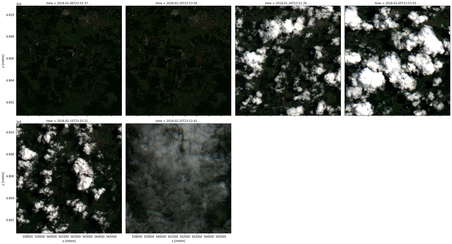
data = product.load(dc, **query)
rgb(data, col='time')
We will need the fmask band too if we want cloud-free images. However, fmask has a different resolution so the following does not work:
[11]:
product = catalog.s2a_nbart_rgb_and_fmask
product
[11]:
measurements:
- nbart_blue
- nbart_green
- nbart_red
- fmask
product: ga_s2am_ard_3
[12]:
try:
    data = product.load(dc, **query)
except ValueError as e:
    print(e, file=sys.stderr)
Not all bands share the same pixel grid
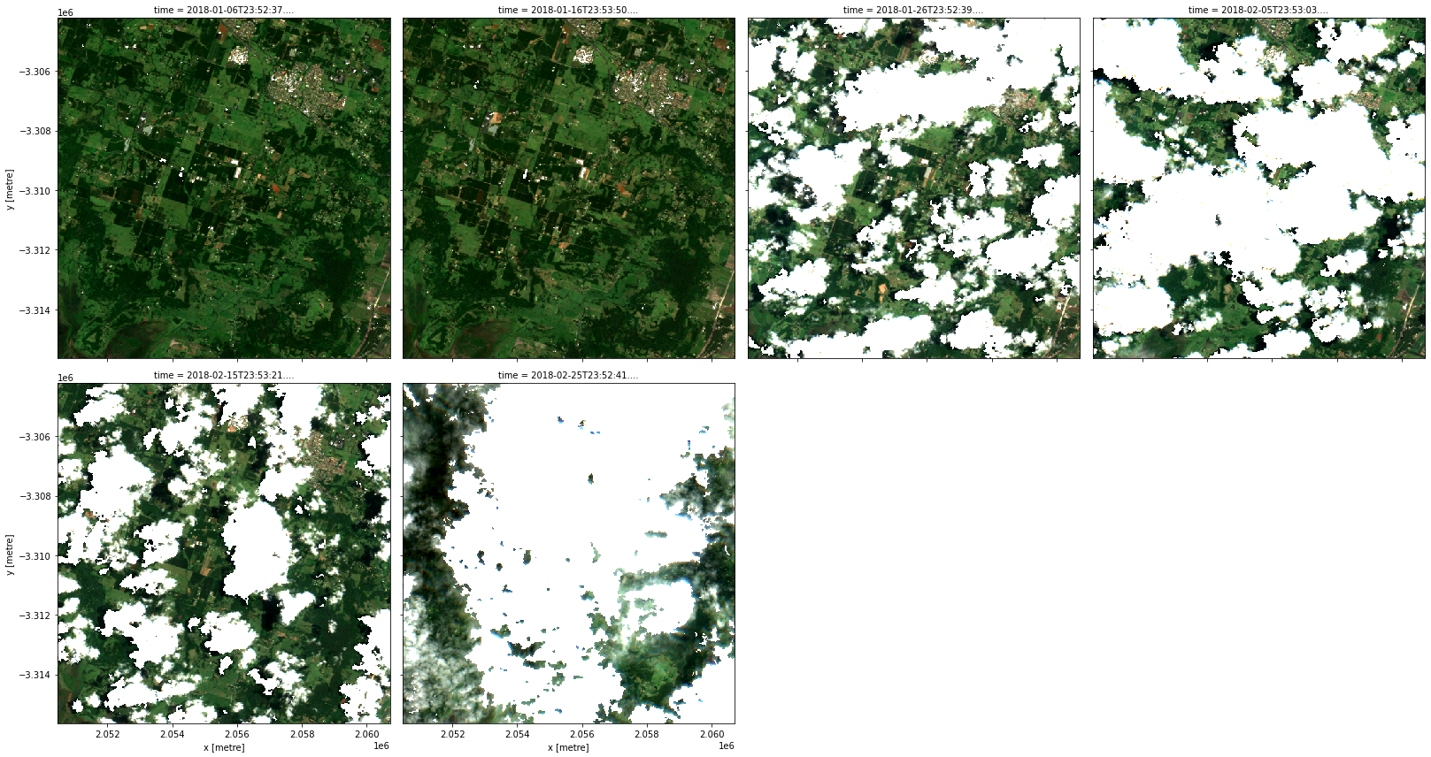
In general, to load datasets from a product that is not “ingested”, such as those in ga_s2am_ard_3, datacube needs to be provided with the output_crs and resolution (and possibly align for sub-pixel alignment).
Note: In this notebook so far we have got away without specifying these. This is because the area of interest we chose happens to contain datasets from only one CRS (coordinate reference system), and the virtual product engine could figure out what grid specification to use. See sections on reprojecting and native load later on in this notebook for more on this.
We can set these in the virtual product so not to repeat ourselves:
[13]:
product = catalog.s2a_nbart_rgb_and_fmask_albers
product
[13]:
measurements:
- nbart_blue
- nbart_green
- nbart_red
- fmask
output_crs: EPSG:3577
product: ga_s2am_ard_3
resampling:
  '*': average
  fmask: nearest
resolution:
- -20
- 20
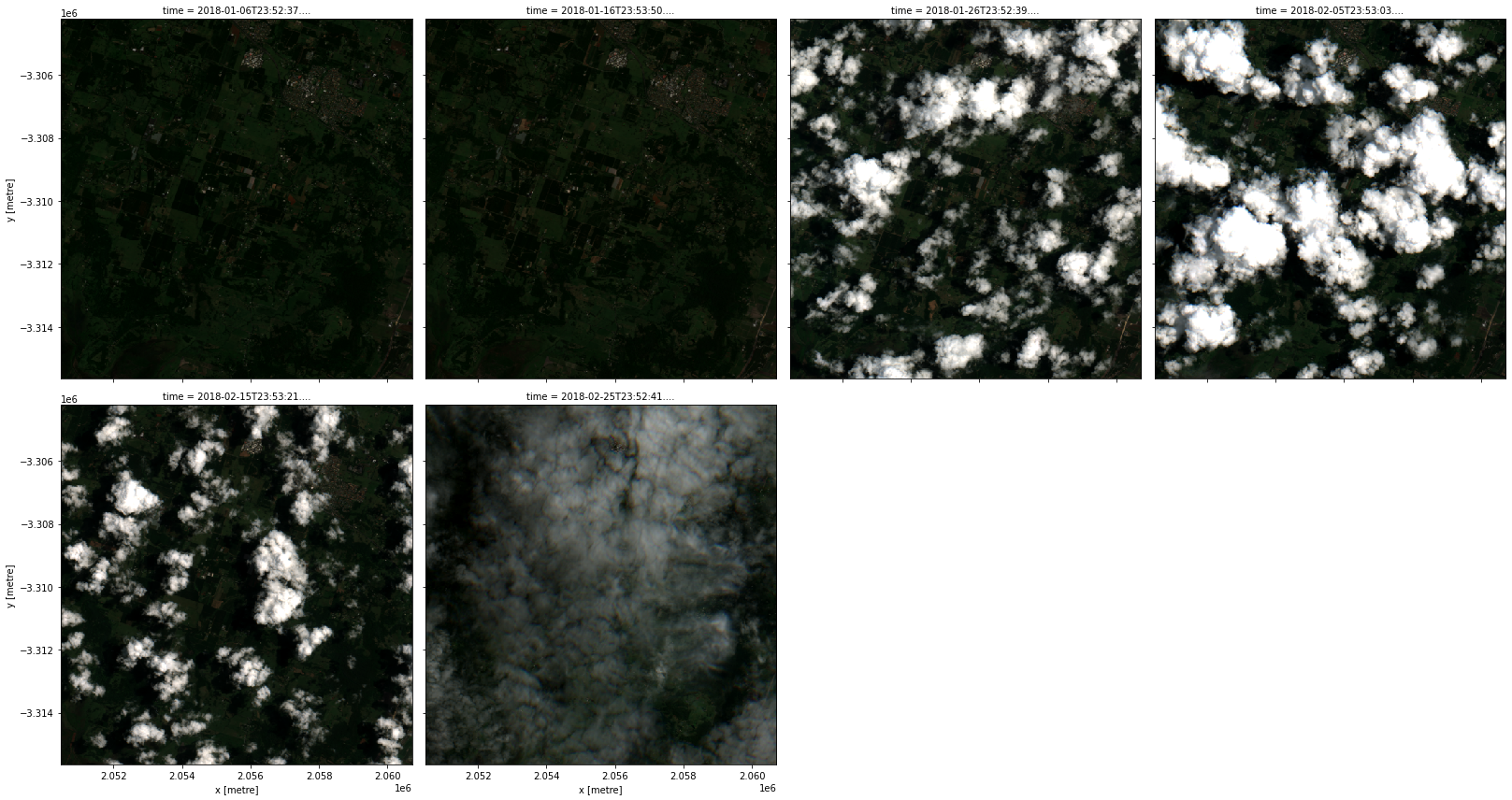
[14]:
# We do not need to specify output crs or resolution here because the product does it for us
data = product.load(dc, **query)
rgb(data, col='time', col_wrap=4)
Data transformations
Cloud-free NBART
So now that we have got the fmask measurement (i.e. band), we can mask out the cloud. First, let’s create the mask that only keeps the valid pixels.
[15]:
product = catalog.s2a_fmask
product
[15]:
flags:
  fmask: valid
input:
  measurements:
  - fmask
  product: ga_s2am_ard_3
mask_measurement_name: fmask
transform: datacube.virtual.transformations.MakeMask
[16]:
data = product.load(dc, **query)
data
[16]:
<xarray.Dataset>
Dimensions:      (time: 6, y: 501, x: 441)
Coordinates:
  * time         (time) datetime64[ns] 2018-01-06T23:52:37.461000 ... 2018-02...
  * y            (y) float64 6.811e+06 6.811e+06 ... 6.801e+06 6.801e+06
  * x            (x) float64 5.370e+05 5.371e+05 ... 5.458e+05 5.458e+05
    spatial_ref  int32 32756
Data variables:
    fmask        (time, y, x) bool True True True True ... False False False
Attributes:
    crs:           epsg:32756
grid_mapping: spatial_refWe now have an fmask band as a boolean mask we want to apply.
Notice that the recipe this time specifies a transform to be applied (datacube.virtual.transformations.MakeMask, which is referred to by its short name make_mask in the file virtual-product-catalog.yaml). That transformation takes certain parameters (flags and mask_measurement_name in this case). It also needs the input, which is this case is the fmask band from the ga_s2am_ard_3 product. You can have other virtual products as input too.
The next step is to apply it to the rest of the bands.
[17]:
product = catalog.s2a_cloud_free_nbart_rgb_albers
product
[17]:
input:
  flags:
    fmask: valid
  input:
    measurements:
    - nbart_blue
    - nbart_green
    - nbart_red
    - fmask
    output_crs: EPSG:3577
    product: ga_s2am_ard_3
    resampling:
      '*': average
      fmask: nearest
    resolution:
    - -20
    - 20
  mask_measurement_name: fmask
  transform: datacube.virtual.transformations.MakeMask
mask_measurement_name: fmask
preserve_dtype: false
transform: datacube.virtual.transformations.ApplyMask
[18]:
data = product.load(dc, **query)
rgb(data, col='time', col_wrap=4)
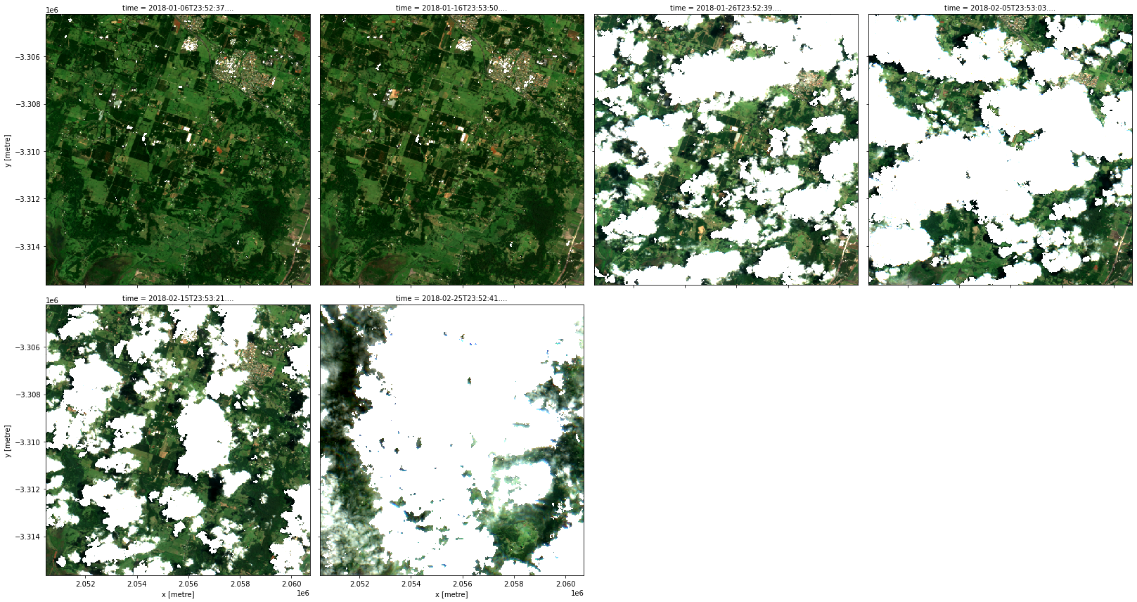
This time there were two (nested) applications of transforms. The outer transform apply_mask (i.e. datacube.virtual.transformations.ApplyMask) took as input the result of the inner transform make_mask (i.e. datacube.virtual.transformations.MakeMask) that was applied, in turn, to the Albers projected NBART bands. Just like mathematical function applications, this recipe too can be read inside out (or right to left) as a data transformation pipeline: we started from our
customized ga_s2am_ard_3 product, then we applied the make_mask transform to it, and then we applied the apply_mask transform to its output.
You could give apply_mask any boolean band (specified by mask_measurement_name) to apply, even if it is not created using make_mask.
Note: The recipe this time was pretty verbose. One advantage of using one catalog for many related virtual products is that parts of their recipes can be shared using some YAML features called anchors and references. See the recipe for the
s2a_cloud_free_nbart_rgb_albersproduct that we just used in thevirtual-product-catalog.yamlfile (view on GitHub). In this case, we recognize that theinputto the transform is just the products2a_nbart_rgb_and_fmask_albersthat we had defined earlier.
Dilation of masks
The make_mask transform optionally can take an argument called dilation that specifies additional buffer for the mask in pixel units. The following recipe is essentially the same as that for s2a_cloud_free_nbart_rgb_albers except for the dilation set to 10 pixels.
[19]:
product = catalog.s2a_cloud_free_nbart_rgb_albers_dilated
product
[19]:
dilation: 10
input:
  flags:
    fmask: valid
  input:
    measurements:
    - nbart_blue
    - nbart_green
    - nbart_red
    - fmask
    output_crs: EPSG:3577
    product: ga_s2am_ard_3
    resampling:
      '*': average
      fmask: nearest
    resolution:
    - -20
    - 20
  mask_measurement_name: fmask
  transform: datacube.virtual.transformations.MakeMask
mask_measurement_name: fmask
preserve_dtype: false
transform: datacube.virtual.transformations.ApplyMask
[20]:
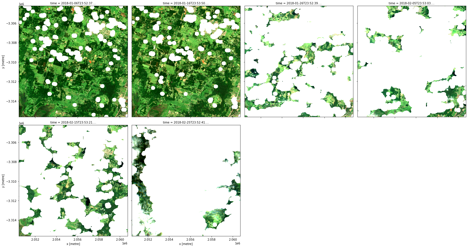
data = product.load(dc, **query)
rgb(data, col='time', col_wrap=4)
Band math
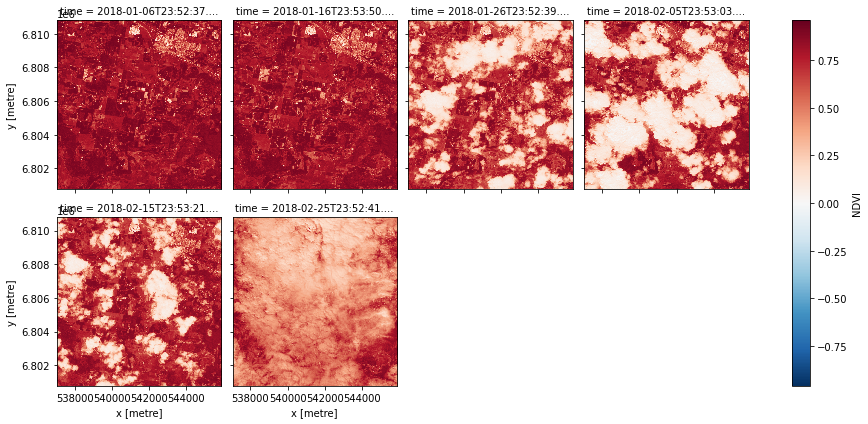
One particularly useful transformation is called expressions (i.e. datacube.virtual.transformations.Expressions) which allows us to use Python arithmetic on bands.
[21]:
product = catalog.s2a_NDVI
product
[21]:
input:
  measurements:
  - nbart_red
  - nbart_nir_1
  product: ga_s2am_ard_3
output:
  NDVI:
    dtype: float32
    formula: (nbart_nir_1 - nbart_red) / (nbart_nir_1 + nbart_red)
transform: datacube.virtual.transformations.Expressions
[22]:
data = product.load(dc, **query)
data.NDVI.plot.imshow(col='time', col_wrap=4)
[22]:
<xarray.plot.facetgrid.FacetGrid at 0x7f230ceb2580>

In a similar fashion, we can define a virtual product that calculates the Tasseled Cap indices too.
[23]:
product = catalog.s2a_tasseled_cap
product
[23]:
input:
  measurements:
  - nbart_blue
  - nbart_green
  - nbart_red
  - nbart_nir_1
  - nbart_swir_2
  - nbart_swir_3
  output_crs: EPSG:3577
  product: ga_s2am_ard_3
  resampling: average
  resolution:
  - -20
  - 20
output:
  brightness:
    dtype: float32
    formula: 0.2043 * nbart_blue + 0.4158 * nbart_green + 0.5524 * nbart_red + 0.5741
      * nbart_nir_1 + 0.3124 * nbart_swir_2 + -0.2303 * nbart_swir_3
  greenness:
    dtype: float32
    formula: -0.1603 * nbart_blue + -0.2819 * nbart_green + -0.4934 * nbart_red +
      0.7940 * nbart_nir_1 + -0.0002 * nbart_swir_2 + -0.1446 * nbart_swir_3
  wetness:
    dtype: float32
    formula: 0.0315 * nbart_blue + 0.2021 * nbart_green + 0.3102 * nbart_red + 0.1594
      * nbart_nir_1 + -0.6806 * nbart_swir_2 + -0.6109 * nbart_swir_3
transform: datacube.virtual.transformations.Expressions
[24]:
data = product.load(dc, **query)
rgb(data, bands=['brightness', 'greenness', 'wetness'], col='time', col_wrap=4)
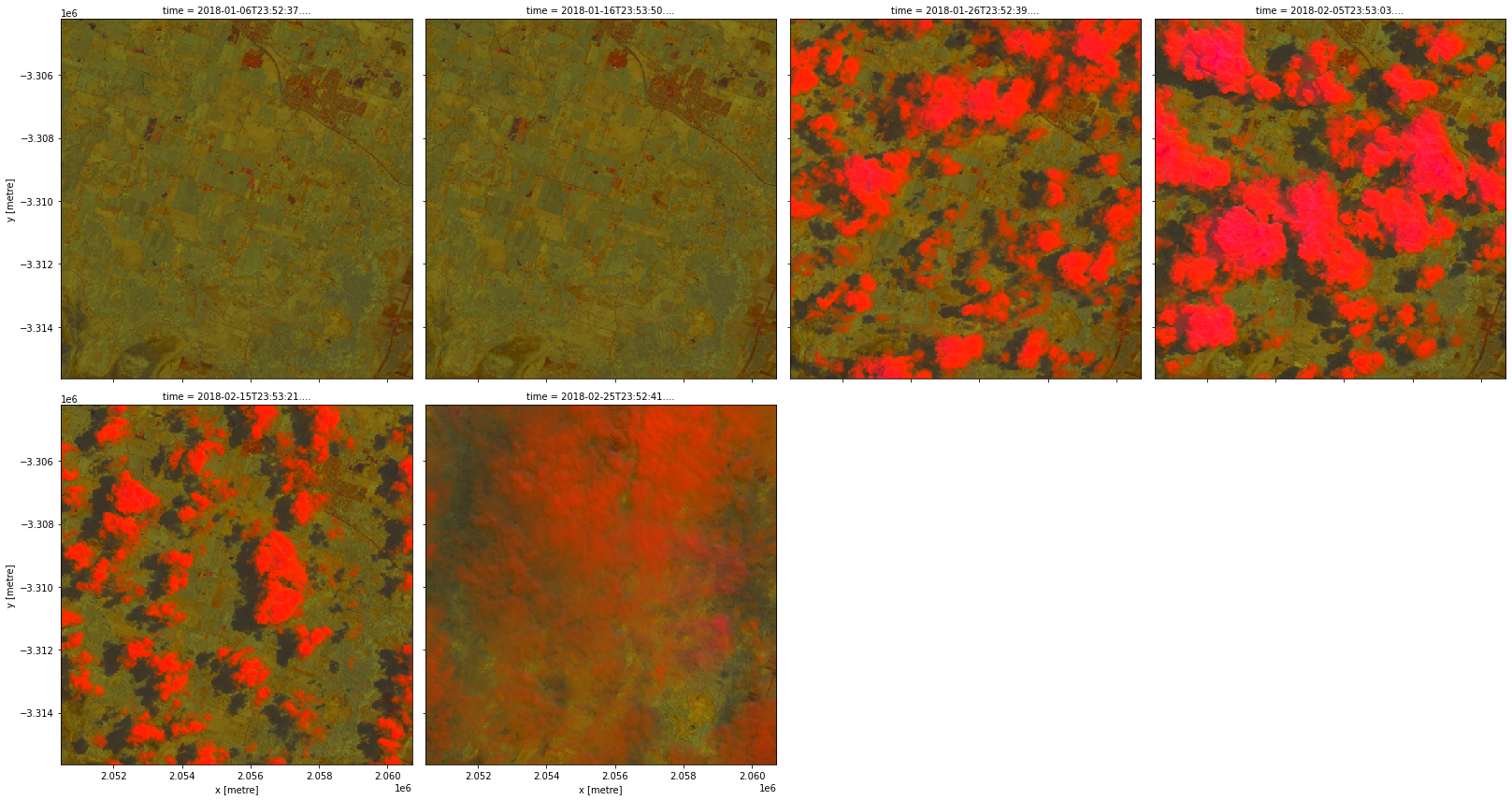
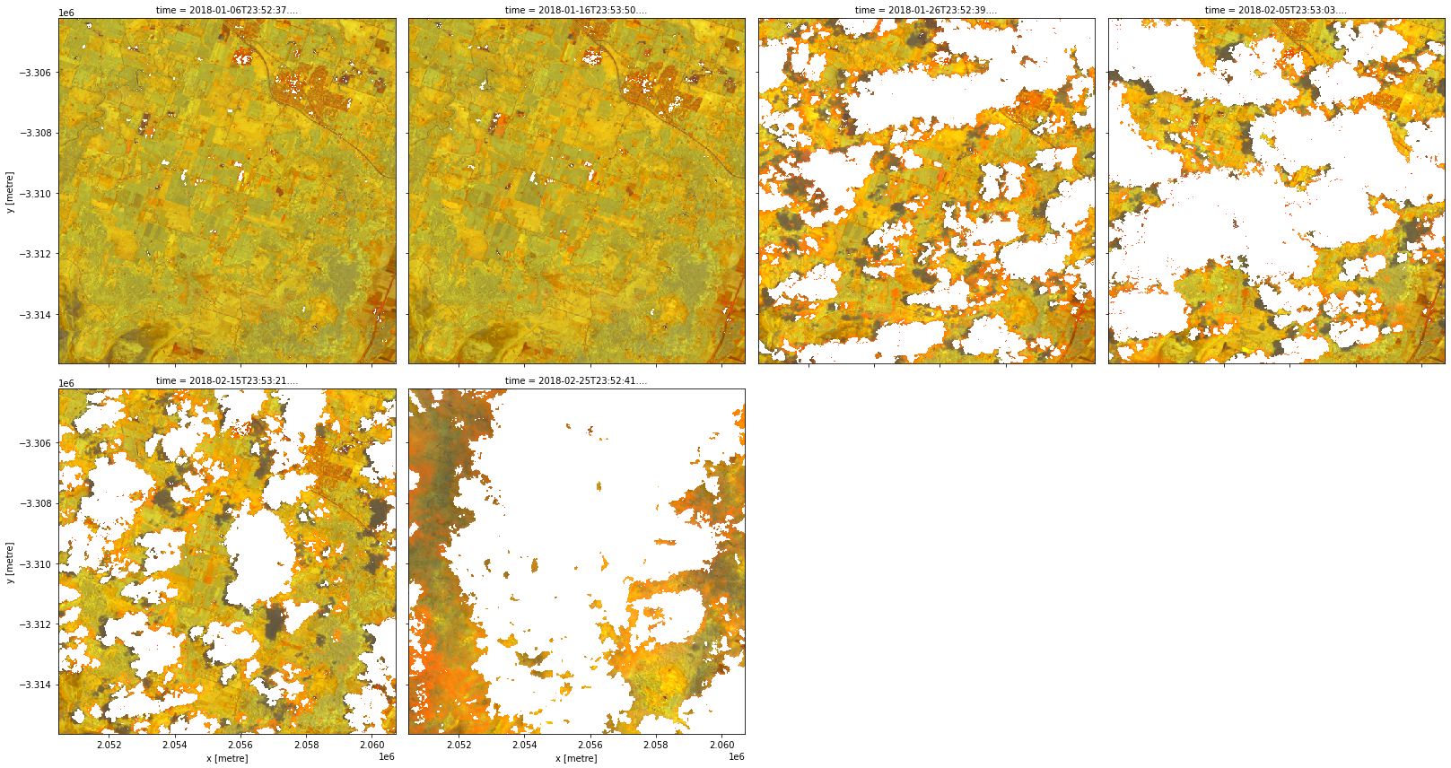
The cloud-free version would probably be more useful for analysis.
[25]:
product = catalog.s2a_cloud_free_tasseled_cap
product
[25]:
input:
  input:
    flags:
      fmask: valid
    input:
      measurements:
      - nbart_blue
      - nbart_green
      - nbart_red
      - nbart_nir_1
      - nbart_swir_2
      - nbart_swir_3
      - fmask
      output_crs: EPSG:3577
      product: ga_s2am_ard_3
      resampling:
        '*': average
        fmask: nearest
      resolution:
      - -20
      - 20
    mask_measurement_name: fmask
    transform: datacube.virtual.transformations.MakeMask
  mask_measurement_name: fmask
  transform: datacube.virtual.transformations.ApplyMask
output:
  brightness:
    dtype: float32
    formula: 0.2043 * nbart_blue + 0.4158 * nbart_green + 0.5524 * nbart_red + 0.5741
      * nbart_nir_1 + 0.3124 * nbart_swir_2 + -0.2303 * nbart_swir_3
  greenness:
    dtype: float32
    formula: -0.1603 * nbart_blue + -0.2819 * nbart_green + -0.4934 * nbart_red +
      0.7940 * nbart_nir_1 + -0.0002 * nbart_swir_2 + -0.1446 * nbart_swir_3
  wetness:
    dtype: float32
    formula: 0.0315 * nbart_blue + 0.2021 * nbart_green + 0.3102 * nbart_red + 0.1594
      * nbart_nir_1 + -0.6806 * nbart_swir_2 + -0.6109 * nbart_swir_3
transform: datacube.virtual.transformations.Expressions
[26]:
data = product.load(dc, **query)

rgb(data, bands=['brightness', 'greenness', 'wetness'], col='time', col_wrap=4)
Combining sensors
To combine multiple sensors into one virtual product, we can use the collate combinator.
[27]:
product = catalog.s2_nbart_rgb
product
[27]:
collate:
- measurements:
  - nbart_blue
  - nbart_green
  - nbart_red
  product: ga_s2am_ard_3
- measurements:
  - nbart_blue
  - nbart_green
  - nbart_red
  product: ga_s2bm_ard_3
[28]:
data = product.load(dc, **query)
rgb(data, col='time', col_wrap=4)
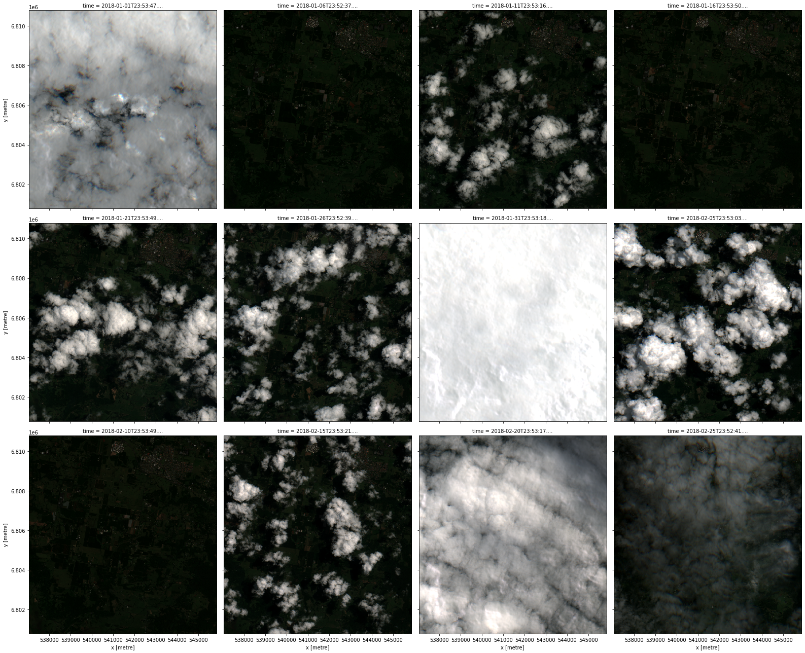
You can collate any number of virtual products as long as they share the same set of measurements.
More advanced usage
Dask
Dask is a useful tool when working with large analyses (either in space or time) as it breaks data into manageable chunks that can be easily stored in memory. It can also use multiple computing cores to speed up computations.
To load virtual products using Dask, pass the dask_chunks specification to the load method.
Note: For more information about using Dask, refer to the Parallel processing with Dask notebook.
[29]:
data = catalog.s2a_NDVI.load(dc, dask_chunks={'time': 1, 'x': 2000, 'y': 2000}, **query)
data
[29]:
<xarray.Dataset>
Dimensions:      (time: 6, y: 1001, x: 882)
Coordinates:
  * time         (time) datetime64[ns] 2018-01-06T23:52:37.461000 ... 2018-02...
  * y            (y) float64 6.811e+06 6.811e+06 ... 6.801e+06 6.801e+06
  * x            (x) float64 5.37e+05 5.371e+05 ... 5.458e+05 5.459e+05
    spatial_ref  int32 32756
Data variables:
    NDVI         (time, y, x) float32 dask.array<chunksize=(1, 1001, 882), meta=np.ndarray>
Attributes:
    crs:           epsg:32756
grid_mapping: spatial_ref[30]:
data.compute().NDVI.plot.imshow(col='time', col_wrap=4)
[30]:
<xarray.plot.facetgrid.FacetGrid at 0x7f22f7e19730>

Statistics
Virtual products support some statistics out-of-the-box (those supported by xarray methods). Here we calculate the mean image of our area of interest. Grouping by year here groups all the data together since our specified time range falls within a year.
[31]:
product = catalog.s2a_mean
product
[31]:
aggregate: datacube.virtual.transformations.XarrayReduction
group_by: datacube.virtual.transformations.year
input:
  input:
    flags:
      fmask: valid
    input:
      measurements:
      - nbart_blue
      - nbart_green
      - nbart_red
      - fmask
      output_crs: EPSG:3577
      product: ga_s2am_ard_3
      resampling:
        '*': average
        fmask: nearest
      resolution:
      - -20
      - 20
    mask_measurement_name: fmask
    transform: datacube.virtual.transformations.MakeMask
  mask_measurement_name: fmask
  preserve_dtype: false
  transform: datacube.virtual.transformations.ApplyMask
method: mean
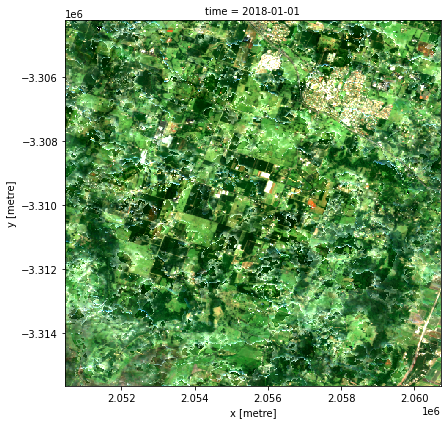
[32]:
data = product.load(dc, **query)
rgb(data, col='time', col_wrap=4)
User-defined transformations
We can define transformations ourselves too. For illustrative purposes, we define the NDVI transform here again, in Python. However, this example is going to be a little bit different since the catalog cannot possibly know about the transformation we are going to define here in the notebook.
Our transformation needs to inherit from datacube.virtual.Transformation and to implement the methods defined there. The construct method is a lower-level way of constructing a virtual product. We will need it since we are going to refer to a Python class directly.
[33]:
from datacube.virtual import Transformation
from datacube.virtual import Measurement
from datacube.virtual import construct


class NDVI(Transformation):

    def compute(self, data):
        return (((data.nbart_nir_1 - data.nbart_red) /
                 (data.nbart_nir_1 + data.nbart_red))
                .astype('float32')
                .to_dataset(name='NDVI'))

    def measurements(self, input_measurements):
        return {'NDVI': Measurement(name='NDVI', dtype='float32', units='1')}


product = construct(transform=NDVI,
                    input=construct(product='ga_s2am_ard_3',
                                    measurements=['nbart_red', 'nbart_nir_1']))
[34]:
data = product.load(dc, **query)
data.NDVI.plot.imshow(col='time', col_wrap=4)
[34]:
<xarray.plot.facetgrid.FacetGrid at 0x7f22f45333d0>
Note that this version does not mask nodata like the expressions version from before automatically does.
Bonus features
Renaming bands
The recipe for the expressions transform, besides the transform and input entries common to all transfoms, contains the output specification, which is a dictionary mapping output band names as keys to recipes for calculating those bands as values. These recipes can themselves be a dictionary as before, containing a formula and optionally specifying a dtype, a nodata value, and a units annotation. They can also be the name of an input band, in
which case the input band is copied unaltered. We can therefore use the expressions transform to copy bands, rename bands, or even drop bands simply by not including it in the output section.
[35]:
product = catalog.s2a_nbart_rgb_renamed
product
[35]:
input:
  measurements:
  - nbart_blue
  - nbart_green
  - nbart_red
  product: ga_s2am_ard_3
output:
  blue: nbart_blue
  green: nbart_green
  red: nbart_red
transform: datacube.virtual.transformations.Expressions
[36]:
data = product.load(dc, **query)
data
[36]:
<xarray.Dataset>
Dimensions:      (time: 6, y: 1001, x: 882)
Coordinates:
  * time         (time) datetime64[ns] 2018-01-06T23:52:37.461000 ... 2018-02...
  * y            (y) float64 6.811e+06 6.811e+06 ... 6.801e+06 6.801e+06
  * x            (x) float64 5.37e+05 5.371e+05 ... 5.458e+05 5.459e+05
    spatial_ref  int32 32756
Data variables:
    blue         (time, y, x) int16 211 203 217 296 304 ... 902 821 820 846 946
    green        (time, y, x) int16 430 388 425 522 516 ... 1119 1191 1273 1317
    red          (time, y, x) int16 227 202 222 339 339 ... 1273 1330 1312 1365
Attributes:
    crs:           epsg:32756
grid_mapping: spatial_refMasking invalid data
The data loaded by datacube usually have a nodata value specified. Often, we want it to be replaced with the NaN value. Since the expressions transform is nodata-aware, we get the same effect just by asking the expressions transform to convert the band to float.
[37]:
product = catalog.s2a_nbart_rgb_nodata_masked
product
[37]:
input:
  measurements:
  - nbart_blue
  - nbart_green
  - nbart_red
  product: ga_s2am_ard_3
output:
  blue:
    dtype: float32
    formula: nbart_blue
  green:
    dtype: float32
    formula: nbart_green
  red:
    dtype: float32
    formula: nbart_red
transform: datacube.virtual.transformations.Expressions
[38]:
data = product.load(dc, **query)
data
[38]:
<xarray.Dataset>
Dimensions:      (time: 6, y: 1001, x: 882)
Coordinates:
  * time         (time) datetime64[ns] 2018-01-06T23:52:37.461000 ... 2018-02...
  * y            (y) float64 6.811e+06 6.811e+06 ... 6.801e+06 6.801e+06
  * x            (x) float64 5.37e+05 5.371e+05 ... 5.458e+05 5.459e+05
    spatial_ref  int32 32756
Data variables:
    blue         (time, y, x) float32 211.0 203.0 217.0 ... 820.0 846.0 946.0
    green        (time, y, x) float32 430.0 388.0 425.0 ... 1.273e+03 1.317e+03
    red          (time, y, x) float32 227.0 202.0 222.0 ... 1.312e+03 1.365e+03
Attributes:
    crs:           epsg:32756
grid_mapping: spatial_refNative load
This feature is in virtual product only at the moment but not in
Datacube.load. We plan to integrate this there in the future.
If all the datasets to be loaded are in the same CRS and all the bands to be loaded have the same resolution and sub-pixel alignment, virtual products will load them “natively”, that is, in their common grid specification, as we have seen before in this notebook.
Sometimes the datasets to be loaded are all in the same CRS but the bands do not have the same resolution. We can specify which resolution to use by setting the like keyword argument to the name of a band.
[39]:
product = catalog.s2a_nbart_rgb_and_fmask_native
product
[39]:
like: fmask
measurements:
- nbart_blue
- nbart_green
- nbart_red
- fmask
product: ga_s2am_ard_3
resampling:
  '*': average
  fmask: nearest
[40]:
data = product.load(dc, **query)
rgb(data, col='time', col_wrap=4)

Reprojecting on-the-fly
We have so far reprojected our images to Albers first, and then applied our cloud mask to it. For (hopefully) higher spectral fidelity, we may want to apply the cloud mask in the native projection, and subsequently reproject to a common grid to obtain a dataset ready for temporal analysis. The reproject combinator in virtual products allow us to do this.
[41]:
product = catalog.s2a_cloud_free_nbart_rgb_albers_reprojected
product
[41]:
input:
  input:
    flags:
      fmask: valid
    input:
      like: fmask
      measurements:
      - nbart_blue
      - nbart_green
      - nbart_red
      - fmask
      product: ga_s2am_ard_3
      resampling: average
    mask_measurement_name: fmask
    transform: datacube.virtual.transformations.MakeMask
  mask_measurement_name: fmask
  preserve_dtype: false
  transform: datacube.virtual.transformations.ApplyMask
reproject:
  output_crs: EPSG:3577
  resolution:
  - -20
  - 20
resampling: average
[42]:
data = product.load(dc, **query)
rgb(data, col='time', col_wrap=4)
Transforms defined in the catalog
We can also store unapplied transforms in the catalog:
[43]:
catalog.nbart_tasseled_cap_transform
[43]:
output:
  brightness:
    dtype: float32
    formula: 0.2043 * nbart_blue + 0.4158 * nbart_green + 0.5524 * nbart_red + 0.5741
      * nbart_nir_1 + 0.3124 * nbart_swir_2 + -0.2303 * nbart_swir_3
  greenness:
    dtype: float32
    formula: -0.1603 * nbart_blue + -0.2819 * nbart_green + -0.4934 * nbart_red +
      0.7940 * nbart_nir_1 + -0.0002 * nbart_swir_2 + -0.1446 * nbart_swir_3
  wetness:
    dtype: float32
    formula: 0.0315 * nbart_blue + 0.2021 * nbart_green + 0.3102 * nbart_red + 0.1594
      * nbart_nir_1 + -0.6806 * nbart_swir_2 + -0.6109 * nbart_swir_3
transform: expressions
The syntax for these transforms is the same as those of the products, except the input section is ommitted (compare the recipe of the product s2a_tasseled_cap here), so that we can provide the input that we want:
[44]:
product = catalog.nbart_tasseled_cap_transform(catalog.s2a_optical_albers)
product
[44]:
input:
  measurements:
  - nbart_blue
  - nbart_green
  - nbart_red
  - nbart_nir_1
  - nbart_swir_2
  - nbart_swir_3
  output_crs: EPSG:3577
  product: ga_s2am_ard_3
  resampling: average
  resolution:
  - -20
  - 20
output:
  brightness:
    dtype: float32
    formula: 0.2043 * nbart_blue + 0.4158 * nbart_green + 0.5524 * nbart_red + 0.5741
      * nbart_nir_1 + 0.3124 * nbart_swir_2 + -0.2303 * nbart_swir_3
  greenness:
    dtype: float32
    formula: -0.1603 * nbart_blue + -0.2819 * nbart_green + -0.4934 * nbart_red +
      0.7940 * nbart_nir_1 + -0.0002 * nbart_swir_2 + -0.1446 * nbart_swir_3
  wetness:
    dtype: float32
    formula: 0.0315 * nbart_blue + 0.2021 * nbart_green + 0.3102 * nbart_red + 0.1594
      * nbart_nir_1 + -0.6806 * nbart_swir_2 + -0.6109 * nbart_swir_3
transform: datacube.virtual.transformations.Expressions
This resultant product is equivalent to the s2a_tasseled_cap product, but what we have gained here is that the nbart_tasseled_cap_transform is more re-usable and can be applied to other products as long as they provide the nbart_* bands.
Additional information
License: The code in this notebook is licensed under the Apache License, Version 2.0. Digital Earth Australia data is licensed under the Creative Commons by Attribution 4.0 license.
Contact: If you need assistance, please post a question on the Open Data Cube Slack channel or on the GIS Stack Exchange using the open-data-cube tag (you can view previously asked questions here). If you would like to report an issue with this notebook, you can file one on
GitHub.
Last modified: September 2021
Compatible datacube version:
[45]:
print(datacube.__version__)
1.8.6
Tags
Tags: NCI compatible, sandbox compatible, sentinel 2, rgb, virtual products, NDVI, tasseled cap, cloud masking, Dask, image compositing, statistics, pixel quality, combining data, native load, reprojecting