DEA Coastlines

DEA Coastlines

Geoscience Australia Landsat Coastlines Collection 3

Version:

2.1.0 (Latest)

Product types:

Derivative, Vector

Time span:

1988 – 2022

Update frequency:

Yearly

Overview

About

A groundbreaking data product, DEA Coastlines combines satellite data with tidal modelling to map the typical location of the Australian coastline at mean sea level for every year since 1988. Resulting shorelines and detailed rates of change show how beaches, sandspits, river mouths, and tidal flats have grown and eroded over time.

Access the data

For help accessing the data, see the Access tab.

See it on a map

See it on a map

Access the data on AWS

Get the data online

Code examples

Code sample

GitHub repository

Code sample

Web Map Service (WMS)

Get via web service

Web Feature Service (WFS)

Get via web service

Key details

Parent product(s)	Landsat 5, 7, 8 and 9 NBART and Observational Attributes
Collection	Geoscience Australia Landsat Collection 3
DOI	10.26186/116268
Licence	Creative Commons Attribution 4.0 International Licence

Cite this product

Data citation	Bishop-Taylor, R., Nanson, R., Sagar, S., Lymburner, L. (2021). Digital Earth Australia Coastlines. Geoscience Australia, Canberra. https://doi.org/10.26186/116268
Paper citation	Bishop-Taylor, R., Nanson, R., Sagar, S., Lymburner, L. (2021). Mapping Australia's dynamic coastline at mean sea level using three decades of Landsat imagery. Remote Sensing of Environment, 267, 112734. https://doi.org/10.1016/j.rse.2021.112734

Publications

Bishop-Taylor, R., Nanson, R., Sagar, S., Lymburner, L. (2021). Mapping Australia’s dynamic coastline at mean sea level using three decades of Landsat imagery. Remote Sensing of Environment, 267, 112734. Available: https://doi.org/10.1016/j.rse.2021.112734

Nanson, R., Bishop-Taylor, R., Sagar, S., Lymburner, L., (2022). Geomorphic insights into Australia’s coastal change using a national dataset derived from the multi-decadal Landsat archive. Estuarine, Coastal and Shelf Science, 265, p.107712. Available: https://doi.org/10.1016/j.ecss.2021.107712

Bishop-Taylor, R., Sagar, S., Lymburner, L., Alam, I., & Sixsmith, J. (2019). Sub-pixel waterline extraction: Characterising accuracy and sensitivity to indices and spectra. Remote Sensing, 11(24), 2984. Available: https://www.mdpi.com/2072-4292/11/24/2984

Details

Background

Australia has a highly dynamic coastline of over 30,000 km, with over 85% of its population living within 50 km of the coast. This coastline is subject to a wide range of pressures, including extreme weather and climate, sea level rise and human development. Understanding how the coastline responds to these pressures is crucial to managing this region, from social, environmental and economic perspectives.

What this product offers

Digital Earth Australia Coastlines is a continental dataset that includes annual shorelines and rates of coastal change along the entire Australian coastline from 1988 to the present.

The product combines satellite data from Geoscience Australia’s Digital Earth Australia program with tidal modelling to map the most representative location of the shoreline at mean sea level for each year. The product enables trends of coastal retreat and growth to be examined annually at both a local and continental scale, and for patterns of coastal change to be mapped historically and updated regularly as data continues to be acquired. This allows current rates of coastal change to be compared with that observed in previous years or decades.

The ability to map shoreline positions for each year provides valuable insights into whether changes to our coastline are the result of particular events or actions, or a process of more gradual change over time. This information can enable scientists, managers and policy makers to assess impacts from the range of drivers impacting our coastlines and potentially assist planning and forecasting for future scenarios.

Applications

• Monitoring and mapping rates of coastal erosion along the Australian coastline

• Prioritise and evaluate the impacts of local and regional coastal management based on historical coastline change

• Modelling how coastlines respond to drivers of change, including extreme weather events, sea level rise or human development

• Supporting geomorphological studies of how and why coastlines have changed across time

Technical information

DEA Coastlines dataset

The DEA Coastlines product contains five layers:

• Annual shorelines

• Rates of change points

• Coastal change hotspots (1 km)

• Coastal change hotspots (5 km)

• Coastal change hotspots (10 km)

Annual shorelines

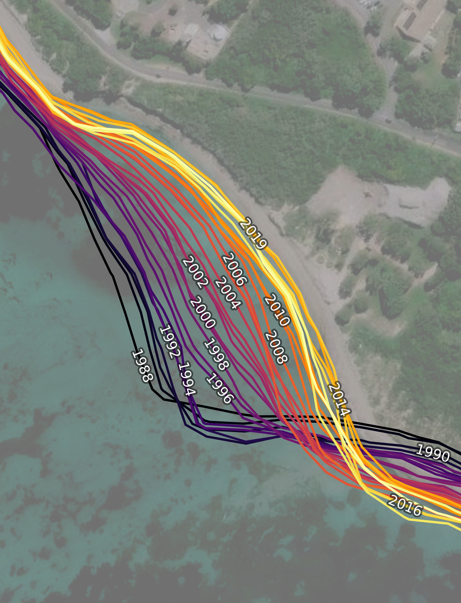
Annual shoreline vectors that represent the median or ‘most representative’ position of the shoreline at approximately 0 m Above Mean Sea Level for each year since 1988 (Figure 1).

Dashed shorelines have low certainty.

Annual shorelines include the following attribute fields:

year	The year of each annual shoreline.
certainty	A column providing important data quality flags for each annual shoreline.
tide_datum	The tide datum of each annual shoreline (e.g. “0 m AMSL”).
id_primary	The name of the annual shoreline’s Primary sediment compartment from the Australian Coastal Sediment Compartments framework.

To understand the certainty field, see the Quality tab.

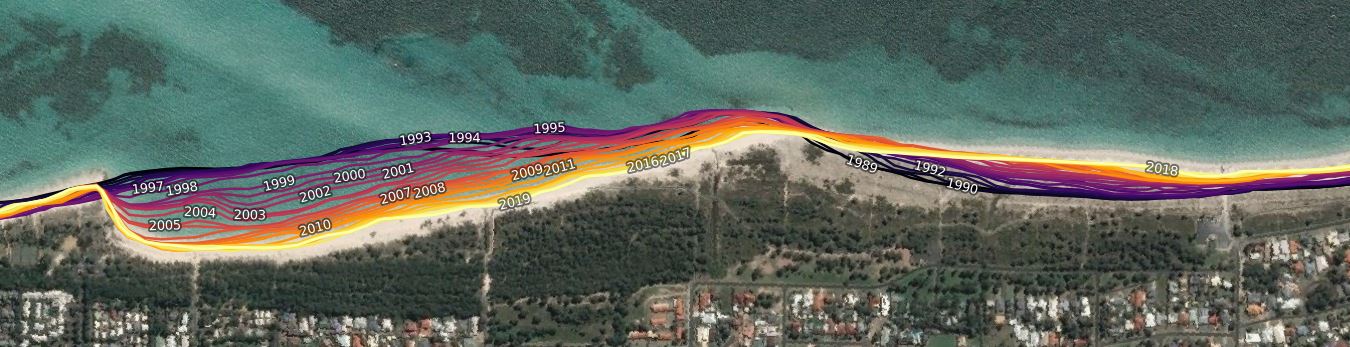
Figure 1: Annual coastlines from DEA Coastlines visualised on the interactive DEA Coastlines web map

Rates of change points

A point dataset providing robust rates of coastal change for every 30 m along Australia’s non-rocky coastlines (Figure 2). The most recent annual shoreline is used as a baseline for measuring rates of change.

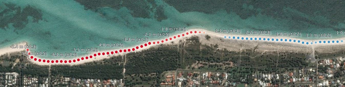
Figure 2: Rates of change points from DEA Coastlines visualised on the interactive DEA Coastlines web map

On the interactive DEA Coastlines web map, points are shown for locations with statistically significant rates of change (p-value <= 0.01; see sig_time below) and good quality data (certainty = “good”; see certainty below) only. Each point shows annual rates of change (in metres per year; see rate_time below), and an estimate of uncertainty in brackets (95% confidence interval; see se_time). For example, there is a 95% chance that a point with a label -10.0 m (±1.0 m) is retreating at a rate of between -9.0 and -11.0 metres per year.

Rates of change points contains the following attribute columns that can be accessed by clicking on labelled points in the web map:

Annual shoreline distances

dist_1990, dist_1991, etc

Annual shoreline distances (in metres) relative to the most recent baseline shoreline. Negative values indicate that an annual shoreline was located inland of the baseline shoreline. By definition, the most recent baseline column will always have a distance of 0 m.

Rates of change statistics

rate_time	Annual rates of change (in metres per year) calculated by linearly regressing annual shoreline distances against time (excluding outliers). Negative values indicate retreat and positive values indicate growth.
sig_time	Significance (p-value) of the linear relationship between annual shoreline distances and time. Small values (e.g. p-value < 0.01 or 0.05) may indicate a coastline is undergoing consistent coastal change through time.
se_time	Standard error (in metres) of the linear relationship between annual shoreline distances and time. This can be used to generate confidence intervals around the rate of change given by rate_time (e.g. 95% confidence interval = se_time * 1.96)
outl_time	Individual annual shoreline are noisy estimators of coastline position that can be influenced by environmental conditions (e.g. clouds, breaking waves, sea spray) or modelling issues (e.g. poor tidal modelling results or limited clear satellite observations). To obtain reliable rates of change, outlier shorelines are excluded using a robust Median Absolute Deviation outlier detection algorithm, and recorded in this column.

Other fields

uid	A unique geohash identifier for each point.
id_primary	The name of the point’s Primary sediment compartment from the Australian Coastal Sediment Compartments framework.
certainty	A column providing important data quality flags for each point in the dataset (see Quality assurance below for more detail about each data quality flag).
sce	Shoreline Change Envelope (SCE). A measure of the maximum change or variability across all annual shorelines, calculated by computing the maximum distance between any two annual shorelines (excluding outliers). This statistic excludes sub-annual shoreline variability.
nsm	Net Shoreline Movement (NSM). The distance between the oldest (1988) and most recent annual shoreline (excluding outliers). Negative values indicate the coastline retreated between the oldest and most recent shoreline; positive values indicate growth. This statistic does not reflect sub-annual shoreline variability, so will underestimate the full extent of variability at any given location.
max_year, min_year	The year that annual shorelines were at their maximum (i.e. located furthest towards the ocean) and their minimum (i.e. located furthest inland) respectively (excluding outliers). This statistic excludes sub-annual shoreline variability.
angle_mean, angle_std	The mean angle and standard deviation between the baseline point to all annual shorelines. This data is used to calculate how well shorelines fall along a consistent line; high angular standard deviation indicates that derived rates of change are unlikely to be correct.
valid_obs, valid_span	The total number of valid (i.e. non-outliers, non-missing) annual shoreline observations, and the maximum number of years between the first and last valid annual shoreline.

Coastal change hotspots (1 km, 5 km, 10 km)

Three points layers summarising coastal change within moving 1 km, 5 km and 10 km windows along the coastline (Figure 3). These layers are useful for visualising regional or continental-scale patterns of coastal change.

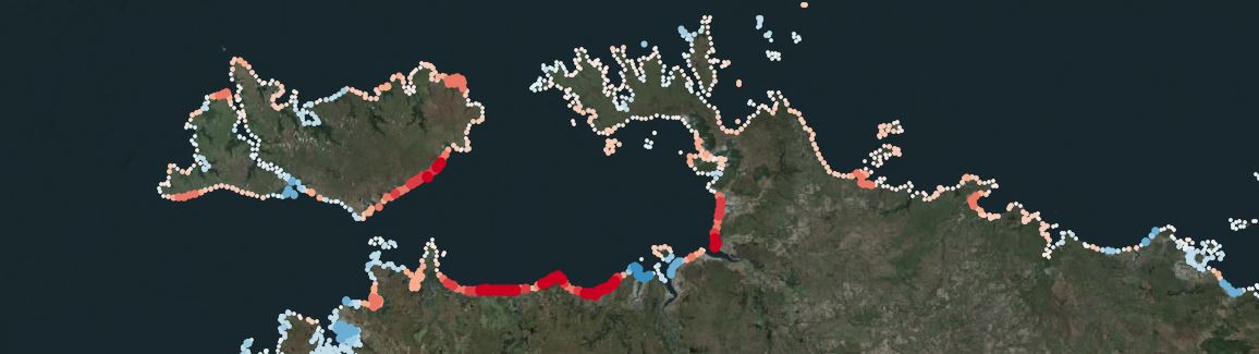
Figure 3: Coastal change hotspots from DEA Coastlines visualised on the interactive DEA Coastlines web map

Processing steps

1. Load stack of all available Landsat 5, 7, 8 and 9 satellite imagery for a location using Digital Earth Australia’s Open Data Cube instance and virtual products.

2. Convert satellite observations to a remote sensing water index (MNDWI; Xu, 2006)

3. For each satellite image, model ocean tides into a 5 x 5 km grid based on exact time of image acquisition using the pixel_tides function from dea_tools

4. Interpolate tide heights into spatial extent of image stack.

5. Mask out high and low tide pixels by removing all observations acquired outside of 50 percent of the observed tidal range centered over mean sea level.

6. Combine tidally-masked data into annual median composites from 1988 to the present representing the coastline at approximately mean sea level.

7. Apply morphological extraction algorithms to mask annual median composite rasters to a valid coastal region.

8. Extract waterline vectors using subpixel waterline extraction (Bishop et al., 2019).

9. Compute rates of coastal change at every 30 m along Australia’s non-rocky coastlines (extracted using the Geoscience Australia Smartline product), and compute linear regression rates of change and derived statistics.

Software

The following software was used to generate this product:

• DEA Coastlines GitHub code

• OpenDataCube

• FES2014 global tide model

References

Bishop-Taylor, R., Nanson, R., Sagar, S., Lymburner, L. (2021). Mapping Australia’s dynamic coastline at mean sea level using three decades of Landsat imagery. Remote Sensing of Environment, 267, 112734. Available: https://doi.org/10.1016/j.rse.2021.112734

Nanson, R., Bishop-Taylor, R., Sagar, S., Lymburner, L., (2022). Geomorphic insights into Australia’s coastal change using a national dataset derived from the multi-decadal Landsat archive. Estuarine, Coastal and Shelf Science, 265, p.107712. Available: https://doi.org/10.1016/j.ecss.2021.107712

Bishop-Taylor, R., Sagar, S., Lymburner, L., & Beaman, R. J. (2019a). Between the tides: Modelling the elevation of Australia’s exposed intertidal zone at continental scale. Estuarine, Coastal and Shelf Science, 223, 115-128. Available: https://doi.org/10.1016/j.ecss.2019.03.006

Bishop-Taylor, R., Sagar, S., Lymburner, L., Alam, I., & Sixsmith, J. (2019b). Sub-pixel waterline extraction: Characterising accuracy and sensitivity to indices and spectra. Remote Sensing, 11(24), 2984. Available: https://doi.org/10.3390/rs11242984

DoT, (2018). Capturing the Coastline: Mapping Coastlines in WA over 75 Years. Department of Transport, Western Australia (2018). Available: https://www.transport.wa.gov.au/mediaFiles/marine/MAC_P_CapturingtheCoastline.pdf

Griffith Centre for Coastal Management, 2016. Sunshine Coast Beach Profile Database: Description of BPA Historical Database and Recommendations for Ongoing Monitoring Programs (No. 188), Griffith Centre for Coastal Management Research Report.

Harrison, A.J., Miller, B.M., Carley, J.T., Turner, I.L., Clout, R., Coates, B., 2017. NSW beach photogrammetry: A new online database and toolbox. Australasian Coasts & Ports 2017: Working with Nature 565.

Lyard, F.H., Allain, D.J., Cancet, M., Carrère, L. and Picot, N., 2021. FES2014 global ocean tide atlas: design and performance. Ocean Science, 17(3), pp.615-649.

Pucino, N., Kennedy, D.M., Carvalho, R.C., Allan, B., Ierodiaconou, D., 2021. Citizen science for monitoring seasonal-scale beach erosion and behaviour with aerial drones. Scientific Reports 11, 3935. https://doi.org/10.1038/s41598-021-83477-6

Sagar, S., Roberts, D., Bala, B., & Lymburner, L. (2017). Extracting the intertidal extent and topography of the Australian coastline from a 28 year time series of Landsat observations. Remote Sensing of Environment, 195, 153-169. Available: https://doi.org/10.1016/j.rse.2017.04.009

Seifi, F., Deng, X. and Baltazar Andersen, O., 2019. Assessment of the accuracy of recent empirical and assimilated tidal models for the Great Barrier Reef, Australia, using satellite and coastal data. Remote Sensing, 11(10), p.1211.

Short, A.D., Bracs, M.A., Turner, I.L., 2014. Beach oscillation and rotation: local and regional response at three beaches in southeast Australia. Journal of Coastal Research 712–717. https://doi.org/10.2112/SI-120.1

South Australian Coast Protection Board, 2000. Monitoring Sand Movements along the Adelaide Coastline. Department for Environment and Heritage, South Australia.

Strauss, D., Murray, T., Harry, M., Todd, D., 2017. Coastal data collection and profile surveys on the Gold Coast: 50 years on. Australasian Coasts & Ports 2017: Working with Nature 1030.

TASMARC, 2021. TASMARC (The Tasmanian Shoreline Monitoring and Archiving Project) (2019) TASMARC database. Available: http://www.tasmarc.info/

Turner, I. L., Harley, M. D., Short, A. D., Simmons, J. A., Bracs, M. A., Phillips, M. S., & Splinter, K. D. (2016). A multi-decade dataset of monthly beach profile surveys and inshore wave forcing at Narrabeen, Australia. Scientific data, 3(1), 1-13. Available: http://narrabeen.wrl.unsw.edu.au/

Xu, H. (2006). Modification of normalised difference water index (NDWI) to enhance open water features in remotely sensed imagery. International journal of remote sensing, 27(14), 3025-3033.

Quality

Accuracy

Annual shoreline accuracy and precision

An extensive validation against independent coastal monitoring datasets was conducted to evaluate the positional accuracy and precision of DEA Coastlines annual shorelines, and the accuracy of our modelled long-term rates of coastal change (i.e. metres retreat or growth per year). In total, 57,662 independent measurements of coastline position were acquired across coastal Australia from the following data sources (Figure 4):

• City of Gold Coast ETA Lines (Strauss et al., 2017)

• Moruya and Pedro Beach survey (Short et al. 2014)

• Narrabeen-Collaroy Beach Survey Program (Turner et al., 2016)

• NSW Beach Profile Database (Harrison et al., 2017)

• South Australia Coastal Monitoring Profile Lines (South Australian Coast Protection Board, 2000)

• Sunshine Coast Council ETA Lines (Griffith Centre for Coastal Management, 2016)

• Tasmanian Shoreline Monitoring and Archiving Project (TASMARC, 2021)

• Victorian Coastal Monitoring Program (Pucino et al., 2021)

• Western Australia Department of Transport (WA DoT) Coastline Movements (Department of Transport, 2009)

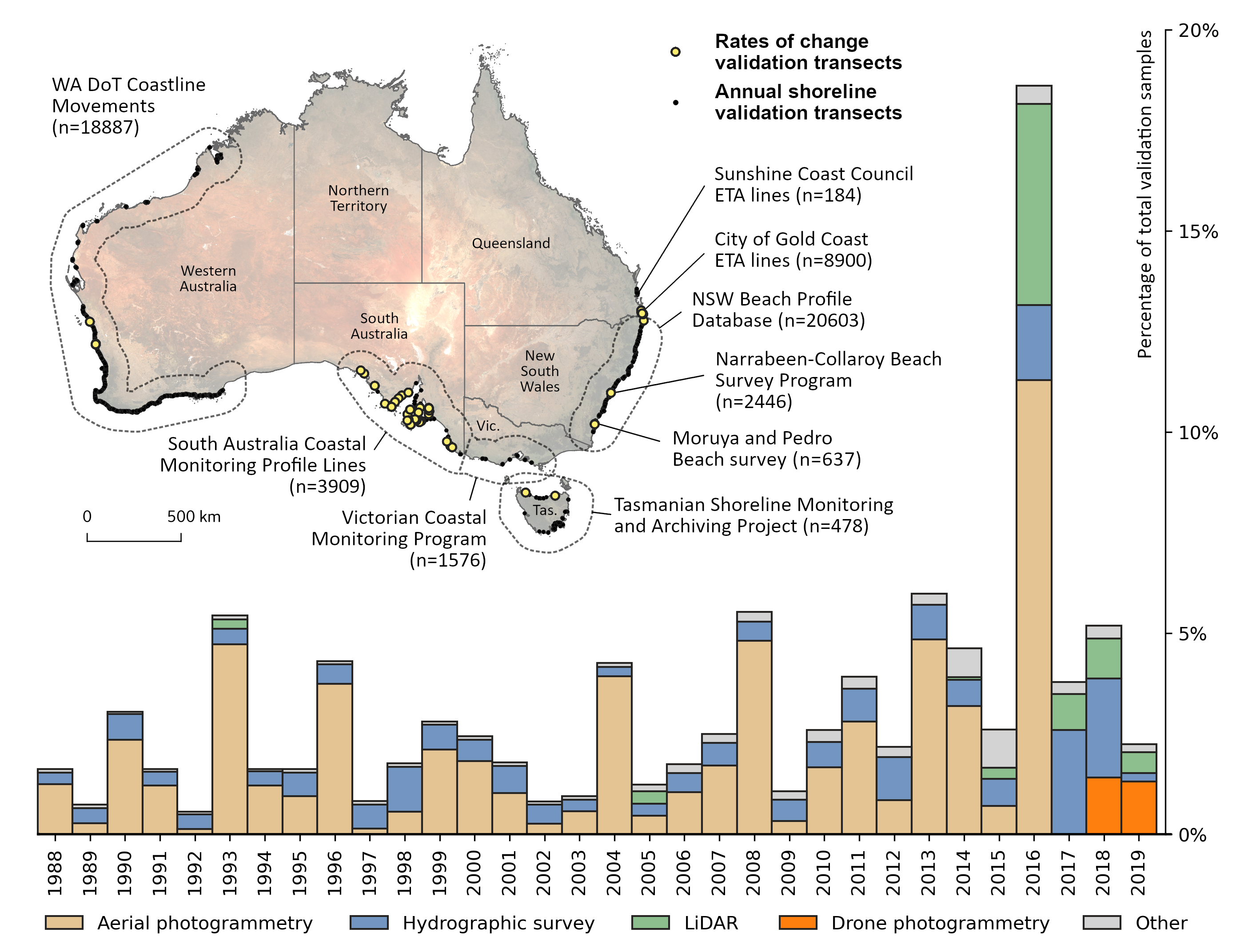
Figure 4: The spatial and temporal distribution of the independent validation data that was compared against DEA Coastlines annual shorelines and rates of change.

Annual shoreline accuracy and precision

This validation assessed the ability of DEA Coastlines to reproduce a specific shoreline proxy: the median annual position of the shoreline at mean sea level (0 m Above Mean Sea Level; AMSL). Validations were performed using existing beach profile lines where possible. For each validation profile line, we identified the median annual position of the 0 m AMSL tide datum across all annual validation observations, and compared this to the position of the corresponding DEA Coastlines shoreline for each year (Figure 5).

To ensure a like-for-like comparison, we selected a subset of validation data with an annual survey frequency approximately equivalent to the Landsat satellite imagery used to generate DEA Coastlines data (i.e. 22 annual observations or greater based on a 16 day overpass frequency). Absolute mapping accuracy (i.e. how far the mapped shorelines were from the median annual position of the shoreline for each year, after correcting for tide) was assessed using Mean Absolute Error (MAE) and Root Mean Squared Error (RMSE):

• Absolute mapping accuracy: 7.3 metres MAE (10.3 metres RMSE) accuracy at mapping the median annual position of the shoreline after correcting for tide

Shoreline mapping bias and precision (i.e. how well modelled shorelines reproduced relative shoreline dynamics even when affected by substrate-specific seaward or landward biases) was evaluated by calculating the average of all individual errors, then subtracting these systematic biases from our results to produce bias-corrected MAE and RMSE. R-squared was also calculated to compare overall correlations between DEA Coastlines and validation shoreline positions:

• Bias: 5.6 metre landward bias (i.e. shorelines mapped inland of their true position)

• Precision: 6.1 metres bias-corrected MAE (8.7 metres bias-corrected RMSE)

• R-squared: 0.92

Learn more: For a more detailed breakdown of validation results by substrate, please refer to Bishop-Taylor et al. 2021.

Rates of change points accuracy

To evaluate our long-term rates of change, we identified 330 validation transects with an extensive (> 10 years) temporal record of coastal monitoring data, encompassing a total of 11,632 independent measurements of shoreline position. We computed linear regression-based annual rates of coastal change (metres per year) between 0 m AMSL shoreline positions and time, and compared these against rates calculated from DEA Coastlines for corresponding years of data to ensure a like-for-like comparison. Validation statistics were then calculated across all 330 transects regardless of statistical significance, and a smaller subset of 144 transects with statistically significant rates of retreat or growth (p < 0.01) in either the validation data or DEA Coastlines:

• All transects:

  • Accuracy: 0.35 m / year MAE (0.60 m / year RMSE)

  • Bias: 0.08 m / year

  • R-squared: 0.90

• Significant transects only:

  • Accuracy: 0.31 m / year MAE (0.52 m / year RMSE)

  • Bias: 0.08 m / year

  • R-squared: 0.95

Learn more: For a more detailed discussion of rates of change validation results, please refer to Bishop-Taylor et al. 2021.

Figure 5: DEA Coastlines annual shorelines compared against a) aerial photogrammetry-derived annual ~0 m AMSL shorelines from the Western Australian Department of Transport Coastline Movements dataset, and b) transect-based in-situ validation data for three example locations that demonstrate sub-pixel precision shoreline extraction: Narrabeen Beach, Tugun Beach, and West Beach. DEA Coastlines transect data in panel b represent the 0 m AMSL Median Annual Shoreline Position shoreline proxy, and have been corrected for consistent local inland biases to assess the ability to capture relative coastline dynamics through time.

Caveats and limitations

Annual shorelines

• Annual shorelines from DEA Coastlines summarise the median (i.e. “dominant”) position of the shoreline throughout the entire year, corrected to a consistent tide height (0 m AMSL). Annual shorelines will therefore not reflect shorter-term coastal variability, for example changes in shoreline position between low and high tide, seasonal effects, or short-lived influences of individual storms. This means that these annual shorelines will show lower variability than the true range of coastal variability observed along the Australian coastline.

Rates of change points

• Rates of change points do not assign a reason for change, and do not necessarily represent processes of coastal erosion or sea level rise. In locations undergoing rapid coastal development, the construction of new inlets or marinas may be represented as hotspots of coastline retreat, while the construction of ports or piers may be represented as hotspots of coastline growth. Rates of change points should therefore be evaluated with reference to the underlying annual coastlines and external data sources or imagery.

• Rates of change points may be inaccurate or invalid within complex mouthbars, or other coastal environments undergoing rapid non-linear change through time. In these regions, it is advisable to visually assess the underlying annual shoreline data when interpreting rates of change to ensure these values are fit-for-purpose. Regions significantly affected by this issue include:

  • Cambridge Gulf, Western Australia

  • Joseph Bonaparte Gulf, Western Australia/Northern Territory

Data quality issues

• Annual shorelines may be less accurate in regions with complex tidal dynamics or large tidal ranges, and low-lying intertidal flats where small tidal modelling errors can lead to large horizontal offsets in coastline positions (Figure 6). Annual shoreline accuracy in intertidal environments may also be reduced by the influence of wet muddy substrate or intertidal vegetation, which can make it difficult to extract a single unambiguous coastline (Bishop-Taylor et al. 2019a, 2019b, 2021). It is anticipated that future versions of this product will show improved results due to integrating more advanced methods for waterline detection in intertidal regions, and through improvements in tidal modelling methods. Regions significantly affected by intertidal issues include:

  • The Pilbara coast, Western Australia from Onslow to Pardoo

  • The Mackay region, Queensland from Proserpine to Broad Sound

  • The upper Spencer Gulf, South Australia from Port Broughton to Port Augusta

  • Western Port Bay, Victoria from Tooradin to Pioneer Bay

  • Hunter Island Group, Tasmania from Woolnorth to Perkins Island

  • Moreton Bay, Queensland from Sandstone Bay to Wellington Point

• Annual shorelines may be noisier and more difficult to interpret in regions with low availability of satellite observations caused by persistent cloud cover. In these regions it can be difficult to obtain the minimum number of clear satellite observations required to generate clean, noise-free annual shorelines. Affected regions include:

  • South-western Tasmania from Macquarie Heads to Southport

• In some urban locations, the spectra of bright white buildings located near the coastline may be inadvertently confused with water, causing a land-ward offset from true shoreline positions.

• Some areas of extremely dark and persistent shadows (e.g. steep coastal cliffs across southern Australia) may be inadvertently mapped as water, resulting in a landward offset from true shoreline positions.

• 1991 and 1992 shorelines are currently affected by aerosol-related issues caused by the 1991 Mount Pinatubo eruption. These shorelines should be interpreted with care, particularly across northern Australia.

Validation approach

• To compare annual shorelines to validation datasets, multiple validation observations in a year were combined into a single median measurement of coastline position. In the case where only a single validation observation was taken for a year, this single observation may not be reflective of typical shoreline conditions across the entire year period. Because of this, validation results are expected to be more reliable for validation datasets with multiple observations per year.

• The current validation approach was biased towards Australia’s south-western, southern and south-eastern coastlines due to the availability of historical coastal monitoring data. This bias prevented us from including more complex intertidal environments in our validation, which is likely to have inflated the accuracy of our results due to issues outlined above.

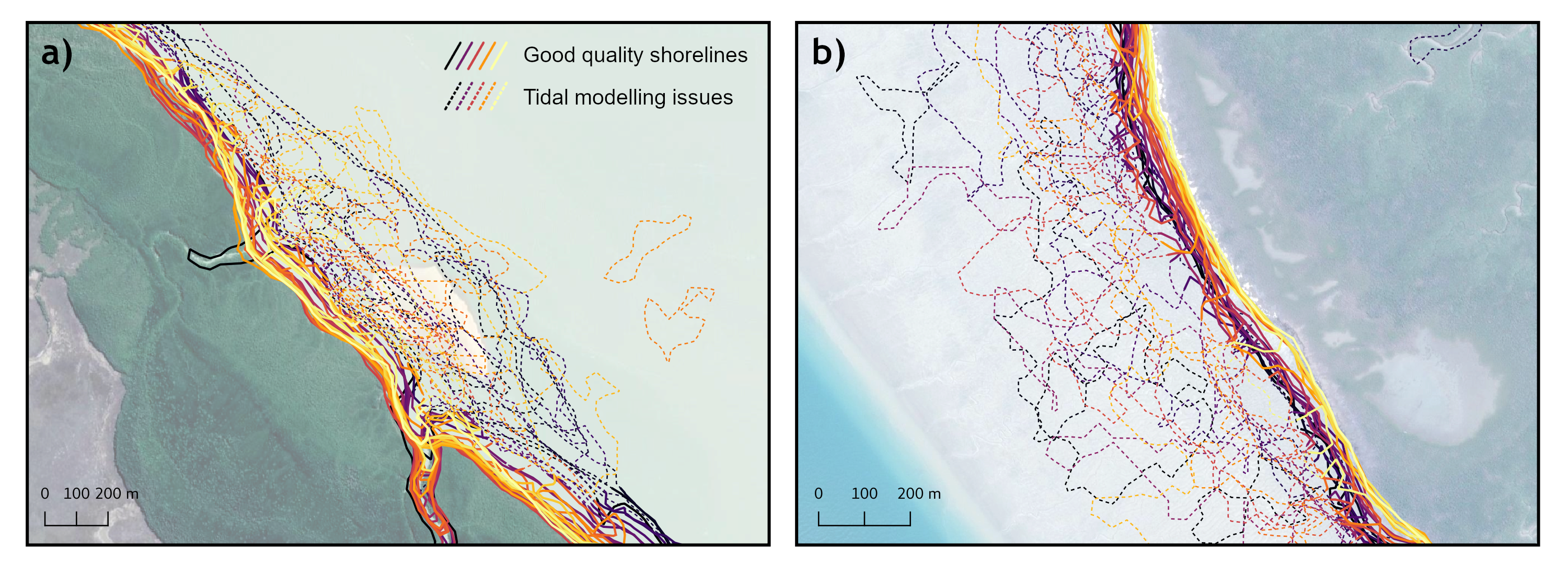
Figure 6: Potentially spurious shorelines in macrotidal coastal regions characterised by gently sloped tidal flat environments: a) Broad Sound and b) Shoalwater Bay, Queensland. Dashed shorelines indicate data that was flagged as affected by tidal modelling issues based on MNDWI standard deviation. In these locations, the TPXO 8 tidal model was unable to effectively sort satellite observations by tide heights, resulting in output shorelines that did not adequately suppress the influence of the tide.

Quality assurance

To allow problematic data to be accounted for or excluded from future analyses, DEA Coastlines data is automatically screened for several potential data quality issues. These issues are flagged in the “certainty” field and symbolised by dashed lines or white points on the interactive DEA Coastlines map. These flags include:

Annual shorelines

• aerosol issues: The accuracy of this shoreline may be affected by aerosol issues caused by the 1991 eruption of Mount Pinatubo.

• insufficient data: The accuracy of this shoreline may be affected by limited good quality satellite observations at this location. This can lead to noisier and less reliable shorelines.

• unstable data: The accuracy of this shoreline is affected by unstable data at this location. This may be caused by errors in the tidal model used to reduce the influence of tide, the presence of gently sloping intertidal mudflats or sandbars that can lead to inaccurate shoreline mapping, or noisy satellite imagery caused by high levels of cloud.

Rates of change points

• insufficient observations: There are insufficient years of good quality annual shoreline data (< 25 years) to calculate reliable rates of coastal change at this location.

• likely rocky shoreline: This coastline has been identified as a probable rocky or cliff shoreline. Rates of coastal change at this location may be less accurate due to noisy shoreline mapping caused by dark terrain shadows.

• extreme value (> 50 m): This location has been identified as having an extreme rate of coastal change (> 50 metres per year) and should be interpreted with caution.

• high angular variability: This rate of coastal change is unlikely to be accurate due to high levels of angular variability from this point to each annual shoreline. This can occur in complex coastal environments like river mouths, sandbars and mudflats that do not show linear patterns of coastal change over time.

• baseline outlier: The baseline (i.e. most recent) annual shoreline is itself flagged as an outlier, potentially resulting in inaccurate rates of change at this location.

Coastal change hotspots

• insufficient points: There are too few valid rates of change points in the 1 km/5 km/10 km radius around this location to calculate a reliable regional rate of change.

For more information, refer to ‘Caveats and limitations’ above.

Access

Access the data

See it on a map	See it on a map	Learn how to use DEA Maps
Get the data online	Access the data on AWS	Learn how to access the data via AWS
Code sample	Code examples GitHub repository	Learn how to use the DEA Sandbox
Get via web service	Web Map Service (WMS) Web Feature Service (WFS)	Learn how to use DEA’s web services

How to access the data

DEA Coastlines data for the entire Australian coastline is available to download in two formats:

• OGC GeoPackage (recommended): suitable for QGIS; includes built-in symbology for easier interpretation

• Esri Shapefiles: suitable for ArcMap and QGIS

To download DEA Coastlines data:

1. Click the Link to data link above

2. Click on either the OGC GeoPackage (coastlines_v2.1.0.gpkg) or Esri Shapefiles (coastlines_v2.1.0.shp.zip) to download the data to your computer.

3. If you downloaded the Esri Shapefiles data, unzip the zip file by right clicking on the downloaded file and selecting Extract all.

To load OGC GeoPackage data in QGIS:

1. Drag and drop the coastlines_v2.1.0.gpkg file into the main QGIS map window, or select it using Layer > Add Layer > Add Vector Layer.

2. When prompted to Select Vector Layers to Add, select all layers and then OK.

3. The DEA Coastlines layers will load with built-in symbology. By default, DEA Coastlines layers automatically transition based on the zoom level of the map. To deactivate this: right click on a layer in the QGIS Layers panel, click Set Layer Scale Visibility, and untick Scale visibility.

How to explore DEA Maps

To explore DEA Coastlines on the interactive DEA Maps platform, visit the link below: https://maps.dea.ga.gov.au/story/DEACoastlines

To add DEA Coastlines to DEA Maps manually:

1. Open DEA Maps.

2. Select Explore map data on the top-left.

3. Select Sea, ocean and coast > DEA Coastlines > DEA Coastlines

4. Click the blue Add to the map button on top-right.

By default, the map will show hotspots of coastal change at continental scale. Red dots represent retreating coastlines (e.g. erosion), while blue dots indicate seaward growth. The larger the dots and the brighter the colour, the more coastal change that is occurring at the location.

More detailed rates of change points will be displayed as you zoom in. To view a time series chart of how a coastal region or area of coastline has changed over time, click on any point (press “Expand” on the pop-up for more detail):

Zoom in further to view individual annual shorelines:

Note: To view a DEA Coastlines layer that is not currently visible (e.g. rates of change points at full zoom), each layer can be added to the map individually from the Sea, ocean and coast > DEA Coastlines > Supplementary data directory.

How to load data from the Web Feature Service (WFS) using Python

DEA Coastlines data can be loaded directly in a Python script or Jupyter Notebook using the DEA Coastlines Web Feature Service (WFS) and geopandas:

import geopandas as gpd

# Specify bounding box
ymax, xmin = -33.65, 115.28
ymin, xmax = -33.66, 115.30

# Set up WFS requests for annual shorelines & rates of change points
deacl_annualshorelines_wfs = f'https://geoserver.dea.ga.gov.au/geoserver/wfs?' \
                       f'service=WFS&version=1.1.0&request=GetFeature' \
                       f'&typeName=dea:shorelines_annual&maxFeatures=1000' \
                       f'&bbox={ymin},{xmin},{ymax},{xmax},' \
                       f'urn:ogc:def:crs:EPSG:4326'
deacl_ratesofchange_wfs = f'https://geoserver.dea.ga.gov.au/geoserver/wfs?' \
                       f'service=WFS&version=1.1.0&request=GetFeature' \
                       f'&typeName=dea:rates_of_change&maxFeatures=1000' \
                       f'&bbox={ymin},{xmin},{ymax},{xmax},' \
                       f'urn:ogc:def:crs:EPSG:4326'

# Load DEA Coastlines data from WFS using geopandas
deacl_annualshorelines_gdf = gpd.read_file(deacl_annualshorelines_wfs)
deacl_ratesofchange_gdf = gpd.read_file(deacl_ratesofchange_wfs)

# Ensure CRSs are set correctly
deacl_annualshorelines_gdf.crs = 'EPSG:3577'
deacl_ratesofchange_gdf.crs = 'EPSG:3577'

# Optional: Keep only rates of change points with "good" certainty
# (i.e. no poor quality flags)
deacl_ratesofchange_gdf = deacl_ratesofchange_gdf.query("certainty == 'good'")

How to load data from the Web Feature Service (WFS) using R

DEA Coastlines data can be loaded directly into R using the DEA Coastlines Web Feature Service (WFS) and the sf package:

library(magrittr)
library(glue)
library(sf)

# Specify bounding box
xmin = 115.28
xmax = 115.30
ymin = -33.66
ymax = -33.65

# Read in DEA Coastlines annual shoreline data, using `glue` to insert our bounding
# box into the string, and `sf` to  load the spatial data from the Web Feature Service
# and set the Coordinate Reference System to Australian Albers (EPSG:3577)
deacl_annualshorelines = "https://geoserver.dea.ga.gov.au/geoserver/wfs?service=WFS&version=1.1.0&request=GetFeature&typeName=dea:shorelines_annual&maxFeatures=1000&bbox={ymin},{xmin},{ymax},{xmax},urn:ogc:def:crs:EPSG:4326" %>%
  glue::glue() %>%
  sf::read_sf() %>%
  sf::st_set_crs(3577)

# Read in DEA Coastlines rates of change points
deacl_ratesofchange = "https://geoserver.dea.ga.gov.au/geoserver/wfs?service=WFS&version=1.1.0&request=GetFeature&typeName=dea:rates_of_change&maxFeatures=1000&bbox={ymin},{xmin},{ymax},{xmax},urn:ogc:def:crs:EPSG:4326" %>%
  glue::glue() %>%
  sf::read_sf() %>%
  sf::st_set_crs(3577)

History

Old versions

No old versions available.

Changelog

2022 DEA Coastlines update

In August 2023, the DEA Coastlines product was updated to version 2.1.0.

This update consists of the addition of annual shoreline data for 2022. The 2022 shoreline is interim data that is subject to change, and will be updated to a final version in the following 2023 DEA Coastlines update (in July 2024).

2021 DEA Coastlines update

In March 2023, the DEA Coastlines product was updated to version 2.0.0. This includes the following key changes to the data and web services:

Improvements and additions:

• Added annual shoreline data for 2021. The 2021 shoreline is interim data that is subject to change, and will be updated to a final version in the following 2022 DEA Coastlines update (in July 2023).

• Improved data coverage over offshore islands and reefs. This includes new shorelines and rates of coastal change over the Indian Ocean, Great Barrier Reef and Coral Sea.

• DEA Coastlines now uses data from the FES2014 global tidal model. This model produces accurate tide modelling across Australia (Seifi et al. 2019) and globally (Lyard et al. 2021) and is more flexible and easier to install than the older TPXO8 tidal model.

• Inclusion of Landsat 9 data to provide additional satellite data from late 2021 onwards.

• Improved shoreline mapping certainty attributes to provide information about the quality of each individual annual shoreline (compared to the previous approach of identifying all annual shorelines in an area as low or good quality; see Quality assurance below for more detail).

• New rates of change points certainty attributes to provide information about the quality of each point (see Quality assurance below for more detail).

• Three coastal change hotspot layers are now included in the product, summarising coastal change within 1 km, 5 km and 10 km windows around each hotspot point. These layers now include attributes providing the median position of all annual shorelines around each hotspot point, which can be used to plot and identify regional trends of coastal change.

• Rates of change points now contain a new “uid” ID field containing a unique geohash ID that can be used to more easily track rates of change points as they are updated in future DEA Coastlines updates.

• Rates of change points include a new “id_primary” field containing the ID of their Primary sediment compartment from the Australian Coastal Sediment Compartments framework. This enables points to be easily queried and summarised by coastal sediment compartment.

Backwards incompatible changes:

• The annual shorelines WFS layer “dea:coastlines” has been renamed to “dea:annual_shorelines”.

• The rates of change points WFS layer “dea:coastlines_statistics” has been renamed to “dea:rates_of_change”.

Previous updates

For a full summary of changes made in previous versions, refer to GitHub.

FAQs

Frequently asked questions

How accurate is DEA Coastlines?

DEA Coastlines shows changes in the median position of the shoreline at mean sea level tide — the position of the shoreline between low and high tide – each year since 1988. This shoreline is accurate to between 7 to 10 metres in a comparison against 57,000 validation data points across the Australian coastline. Rates of coastal change are accurate to between 0.31 to 0.35 metres per year.

This level of accuracy allows the product to accurately map and monitor long-term changes in coastline positions over time at a scale relevant to local and regional coastal management.

The accuracy of DEA Coastlines is lower in complex and dynamic coastal environments such as intertidal flats, river mouths, rapidly changing sand bars, and where muddy substrates, turbid water and large tidal ranges make it difficult to extract a single, clean coastline.

Cloud cover can also reduce the accuracy of the product by reducing the availability of clear satellite imagery. The data can also be limited over remote islands or reefs due to a lack of historical satellite information.

For detailed information about the accuracy and limitations of DEA Coastlines, refer to the Quality tab.

DEA Coastlines 2021 dataset incorporates Landsat 9 data and uses a new tidal model. How might this affect my pre-2020 modelling?

The addition of Landsat 9 satellite data to the underlying source data of DEA Coastlines will affect all annual shorelines from 2021 onwards. The additional data is expected to improve the overall quality of the annual shorelines by providing cleaner and more stable annual layers.

The integration of a new global tidal model (FES2014) may result in minor changes to the product’s historical coastlines and derived rates of coastal change. These changes are likely to be greatest in macrotidal regions of Australia such as north-western Western Australia and central Queensland. A comparison of annual shoreline accuracy at the microtidal Narrabeen Beach in Sydney shows consistent results between DEA Coastlines version 1.1.0 and the newer version 2.0.0.

Where specific changes or issues have been identified, they are noted on this product page.

What causes changing coastlines?

DEA Coastlines presents a historical record of coastal change since 1988 – it does not assign a reason or cause for coastal change or make predictions about future patterns or rates of coastal change.

Coastal change is complex and driven by many interacting factors including local geomorphology (the shape of the local coastline), extreme weather and climatic events such as La Niña, ocean currents, wind patterns, and coastal development.

For example, the construction of new inlets or marinas may be represented in DEA Coastlines as areas of coastline retreat, while the construction of ports or piers may be represented as areas of coastline growth. Rates of change from DEA Coastlines should therefore be evaluated carefully with reference to the underlying annual coastlines, and other more detailed data sources or imagery.

Does DEA Coastlines show the effect of individual storms?

No. DEA Coastlines shows the most representative (median) location of the coastline over an entire year, so does not show the effect of individual major storms. However, DEA Coastlines data can be used to identify coastlines that respond to longer-scale climatic cycles such as El Niño–Southern Oscillation (ENSO). For example, coastlines in eastern Australia may retreat as La Nina conditions increase the likelihood of east coast lows, damaging cyclones and extreme storm surges.

Could DEA Coastlines replace local coastal monitoring surveys?

No. Local on-the-ground and aerial coastal monitoring surveys are still crucial to the management of coastal areas. DEA Coastlines provides an affordable and efficient option for larger-scale planning and for better understanding of long-term coastal trends. Coastal monitoring data provided by local and state government, universities, and citizen science projects has been critical for validating DEA Coastlines.

Credits

Acknowledgments

The authors would like to sincerely thank the following organisations and individuals for providing validation data and valuable feedback on preliminary versions of this product:

• Centre for Integrative Ecology, Deakin University

• Griffith Centre for Coastal Management, Griffith University

• Water Research Laboratory, University of New South Wales

• Victorian Coastal Monitoring Program

• TASMARC Project, Antarctic Climate & Ecosystems Cooperative Research Centre

• City of Gold Coast, Queensland

• Sunshine Coast Council, Queensland

• Western Australia Department of Transport

• South Australia Department of Environment and Water

• Queensland Department of Environment and Science

• NSW Department of Planning, Industry and Environment

• Andrew Short, University of Sydney

• Colin Woodroffe, University of Wollongong

This research was undertaken with the assistance of resources from the National Computational Infrastructure (NCI), which is supported by the Australian Government.

Tidal modelling is provided by the FES2014 global tidal model, implemented using the pyTMD Python package. FES2014 was produced by NOVELTIS, LEGOS, CLS Space Oceanography Division and CNES. It is distributed by AVISO, with support from CNES (http://www.aviso.altimetry.fr/).

License and copyright

© Commonwealth of Australia (Geoscience Australia).

Released under Creative Commons Attribution 4.0 International Licence.