DEA Intertidal
DEA Intertidal
- Version:
- Type:
Derivative, Raster
- Resolution:
10 m
- Coverage:
2016 to 2023
- Data updates:
Yearly frequency, Ongoing
About
The DEA Intertidal product suite maps the changing elevation, exposure and tidal characteristics of Australia’s exposed intertidal zone, the complex zone that defines the interface between land and sea.
Incorporating both Sentinel-2 and Landsat data, the product suite provides an annual 10 m resolution elevation product for the intertidal zone, enabling users to better monitor and understand some of the most dynamic regions of Australia’s coastlines. Utilising an improved tidal modelling capability, the product suite includes a continental scale mapping of intertidal exposure over time, enabling scientists and managers to integrate the data into ecological and migratory species applications and modelling.
Streaming data from AWS is strongly recommended
DEA Intertidal data is extremely large with files up to 15 GB in size. We strongly recommend streaming data directly from the cloud rather than downloading the data. Please see the instructions on the Access tab: How to stream data from AWS
Access the data
For help accessing the data, see the Access tab.
See it on a map
Explore data availability
Download the data from ELVIS
Access the data on NCI
View code examples
GitHub repository
Web Map Service (WMS)
AWS data
How to stream data from AWS
Key specifications
For more specifications, see the Specifications tab.
Technical name |
Geoscience Australia Sentinel-2 Landsat Intertidal Calendar Year Collection 3 |
Bands |
|
DOI |
|
Currency |
|
Parent product |
Sentinel-2A, -2B and -2C and Landsat 7, 8, and 9 NBART and Observational Attributes |
Collections |
Geoscience Australia Landsat Collection 3, Geoscience Australia Sentinel-2 Collection 3 |
Licence |
Cite this product
Data citation |
Bishop-Taylor, R., Phillips, C., Newey, V., Sagar, S. (2024). Digital Earth Australia Intertidal. Geoscience Australia, Canberra. https://dx.doi.org/10.26186/149403
|
Publications
Bishop-Taylor, R., Sagar, S., Lymburner, L., Beaman, R.L., 2019. Between the tides: modelling the elevation of Australia’s exposed intertidal zone at continental scale. Estuarine, Coastal and Shelf Science. Available: https://doi.org/10.1016/j.ecss.2019.03.006
Sagar, S., Phillips, C., Bala, B., Roberts, D., Lymburner, L., 2018. Generating continental scale pixel-based surface reflectance composites in coastal regions with the use of a multi-resolution tidal model. Remote Sensing. 10, 480. Available: https://doi.org/10.3390/rs10030480
Sagar, S., Roberts, D., Bala, B., Lymburner, L., 2017. Extracting the intertidal extent and topography of the Australian coastline from a 28 year time series of Landsat observations. Remote Sensing of Environment 195, 153-169. Available: https://doi.org/10.1016/j.rse.2017.04.009
Background
Intertidal environments contain many important ecological habitats such as sandy beaches, tidal flats, rocky shores, and reefs. These environments also provide many valuable benefits such as storm surge protection, carbon storage, and natural resources.
Intertidal zones are being increasingly faced with threats including coastal erosion, land reclamation (e.g. port construction), and sea level rise. These regions are often highly dynamic, and accurate, up-to-date elevation data describing the changing topography and extent of these environments is needed.
The intertidal zone also forms a critical habitat and foraging ground for migratory shore birds and other species. An improved characterisation of the exposure patterns of these dynamic environments is important to support conservation efforts and to gain a better understanding of migratory species pathways. However, this data is expensive and challenging to map across the entire intertidal zone of a continent the size of Australia.
The DEA Intertidal product suite provides annual continental-scale elevation and exposure product layers for Australia’s exposed intertidal zone, mapped at a 10 m resolution from DEA’s archive of open-source Landsat and Sentinel-2 satellite data. The exposed intertidal zone consists of coastal regions periodically inundated by tidal flows, not including areas obscured by vegetation cover such as mangroves. These intertidal products enable users to better monitor and understand some of the most dynamic regions of Australia’s coastlines.
Applications
Integration with existing topographic and bathymetric data to seamlessly map the elevation of the coastal zone.
Providing baseline elevation data to assist coastal hazard impact assessment from extreme weather and inundation events.
Investigating coastal erosion and sediment transport processes.
Supporting habitat mapping and modelling for coastal ecosystems extending across the terrestrial to marine boundary.
Characterise the spatio-temporal exposure patterns of the intertidal zone to support migratory species studies and applications.
Technical Information
Features
The DEA Intertidal product suite contains 4 core product layers, 7 tidal attribute (ta) layers, and 4 quality assessment (qa) layers, all provided as continental 10 m resolution GeoTIFFs for the Australian coastal and intertidal region.
All datasets are produced annually from a 3-year composite of input data from combined Sentinel-2 and Landsat DEA Collection 3 surface reflectance products. The product time series commences from 2016, with datasets labelled by the middle year of data. For example, the 2017 layer combines data from 2016, 2017, and 2018. Updates to the product suite are scheduled annually.
What this product offers
The DEA Intertidal product suite is the next generation of intertidal products developed in DEA. It improves on the DEA Intertidal Elevation Model (also known as the National Intertidal Digital Elevation Model or NIDEM) (Bishop-Taylor et al., 2019) and adds several new features and products to help users better understand the intertidal environment.
NIDEM was the first 3D model of Australia’s intertidal zone — the area of coastline exposed and flooded by ocean tides. The DEA Intertidal suite fundamentally changes and improves the way in which the exposed intertidal zone is modelled compared to the original NIDEM elevation model:
The addition of Sentinel-2 data improves the spatial resolution of the model to 10 m, compared to the 25m of the original NIDEM.
Incorporation of a new pixel-based method supports a reduction in the temporal epoch of the product to 3 years (in comparison to 28 years in NIDEM), improving the ability to capture the current state of dynamic coastal environments and enabling ‘change over time’ applications using annual epochs.
Quantification of the vertical uncertainty of the elevation model.
An Intertidal Exposure model at 10 m resolution to examine the spatiotemporal patterns of exposure and inundation across the intertidal zone, supporting migratory species studies and habitat mapping applications.
Tidal metrics to enable users to understand the varied ranges and distributions of tidal stages observed by the Landsat and Sentinel-2 satellites across Australia, and how this information can be used to better understand and interpret the products.
The implementation of an ensemble tidal modelling approach, acknowledging the wide range of global and regional tide models available and their varying performance across different regions of Australia. See Ensemble Tidal Modelling.
A coastal extents classification model that identifies five categorical classes to compliment the Elevation and Exposure products. This helps users to characterise different environments in the coastal zone in terms of their inundation characteristics and drivers, mapping confidence and nature of water cover.
File Naming Convention
The file naming convention is as follows:
{Organisation}_{Platform}_{Product}_{Reporting period}_{Collection}_{Tile reference}_{Data date}--{Data period}_{Product status}_{Band name}.{File extension}
Datasets
Annual files for each of the product bands are available in DEA’s Amazon S3 bucket in two formats: 32 km² tiles and continental mosaics. For access and usage information, see the Access tab.
32 km² grid tiles are available as downloadable GeoTIFF files, for example:
ga_s2ls_intertidal_cyear_3_x082y139_2022--P1Y_final_elevation.tif
Single-band annual continental data mosaics are delivered to support access and navigability of DEA Intertidal data in geospatial information system (GIS) environments. These datasets, delivered in cloud-optimised GeoTIFF (COG) format, are recommended for fast and efficient data streaming of single-band layers of the DEA Intertidal product. Here’s an example of the COG file naming convention:
ga_s2ls_intertidal_cyear_3_2017_exposure.tif
Code repositories
DEA Intertidal GitHub repository — A codebase for DEA Intertidal product generation workflows
EO-Tides GitHub repository — A codebase for integrating satellite Earth observations with tide modelling
DEA Tools GitHub repository — Earth observation data manipulation tools
PyTMD GitHub repository — Python-based tidal prediction software
Core Product Layers
See the attributes of these layers in the Specifications tab.
DEA Intertidal Elevation (elevation)
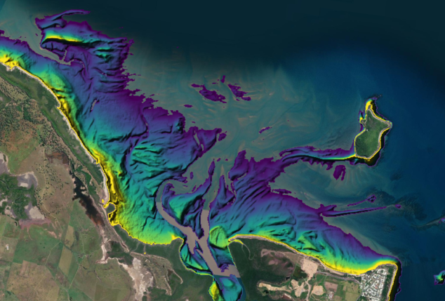
DEA Intertidal Elevation (Figure 1) provides elevation in metre units relative to modelled Mean Sea Level for each pixel of the satellite-observed exposed intertidal zone across the Australian coastline. The elevation model is generated from DEA Landsat and Sentinel-2 surface reflectance data from each 3-year composite period, utilising a pixel-based approach based on Ensemble Tidal Modelling. For every pixel, the time series of surface reflectance data is converted to the Normalised Difference Water Index (NDWI) and each observation tagged with the tidal height modelled at the time of acquisition by the satellite. A rolling median is applied from low to high tide to reduce noise (such as white water, sunglint, and non-tidal water level variability), then analysed to identify the tide height at which the pixel transitions from dry to wet. This tide height represents the elevation of the pixel.
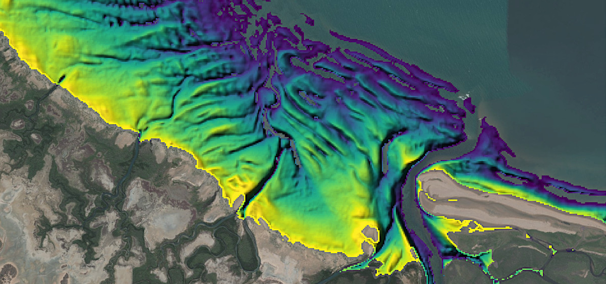
Figure 1. DEA Intertidal Elevation, with low elevation values shown in dark colours and high elevation shown in light colours.
DEA Intertidal Elevation Uncertainty (elevation_uncertainty)
DEA Intertidal Elevation Uncertainty (Figure 2) provides a measure of the quality of each modelled elevation value in metre units. Uncertainty is calculated by assessing how cleanly the modelled elevation separates satellite observations into dry and wet observations. This is achieved by identifying satellite observations that were misclassified by the modelled elevation (for instance, pixels that were observed as wet at tide heights lower than the modelled elevation, or alternately, observed as dry at higher tide heights). The spread of tide heights from these misclassified observations is summarised using a robust Median Absolute Deviation (MAD) statistic, and reported as \(0.5 \times MAD\) to represent one-sided uncertainty bounds (i.e. ± uncertainty on either side of the pixel’s elevation). Common causes of high elevation uncertainty can be poor tidal model performance, rapidly changing intertidal morphology, or noisy underlying satellite data.
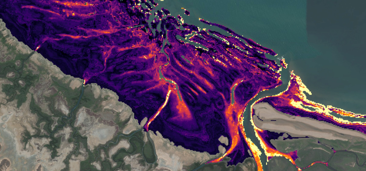
Figure 2. DEA Intertidal Elevation Uncertainty, with high uncertainty shown in light colours.
DEA Intertidal Exposure (exposure)
DEA Intertidal Exposure (Figure 3) models the percentage of time that any intertidal pixel of known elevation is exposed from tidal inundation. Exposure is calculated by comparing the pixel elevation back against a high temporal resolution model of tide heights for that location, based on the Ensemble Tidal Modelling approach. Exposure percentage is calculated as the fraction of exposed observations relative to the total number of observations generated in the high temporal resolution tidal model for the 3-year product epoch.
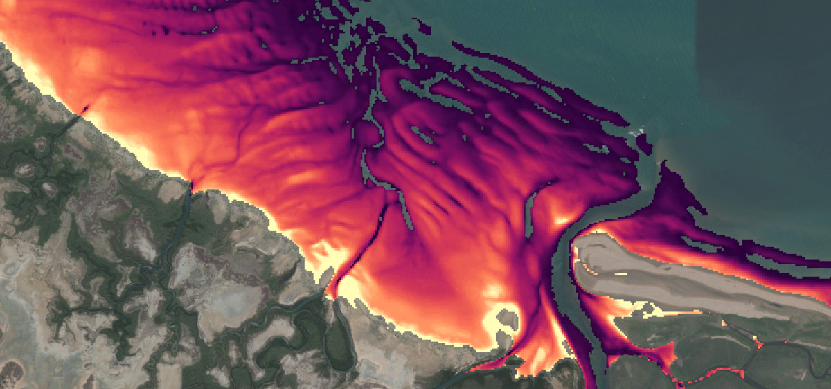
Figure 3. DEA Intertidal Exposure, with low exposure values (i.e. rarely exposed pixels) shown in dark colours.
DEA Intertidal Extents (extents)
DEA Intertidal Extents is a categorical dataset that classifies coastal areas into five classes (Figure 4), including the satellite-observed extents of the exposed (i.e. non-vegetated) intertidal zone. This classification is based on DEA Intertidal Elevation outputs and other satellite-derived data including the inundation frequency of each pixel and correlations between inundation patterns and modelled tide heights. See Quality Assessment Layers. The “intensive urban” land use summary class of the Catchment-scale Land Use Map (CLUM) (ABARES, 2021) dataset was used to mask pixel misclassifications in urban areas.
The class definitions of the Intertidal Extents layer are as follows.
Ocean and coastal waters (1) — Pixels that are wet in 50% or more of satellite observations and are located within the coastal mask (a cost-distance connectivity mask combining elevation with distance from the ocean).
Exposed intertidal - low confidence (2) — Pixels that have a correlation between tide height and NDWI of at least 0.15, and are located within the coastal mask (see Ocean and coastal waters).
Exposed intertidal - high confidence (3) — Pixels that are included in the intertidal elevation dataset.
Inland waters (4) — Pixels that are wet in more than 50% of satellite observations, and fall outside of the coastal mask (see Ocean and coastal waters).
Land (5) — Pixels that are wet in less than 50% of satellite observations.
Figure 4. DEA Intertidal Extents, the five coastal classes include ocean and coastal waters (dark blue), low confidence intertidal (yellow), high confidence intertidal (orange), inland waters (light blue), and land (white).
Tidal Attribute Layers
See the attributes of these layers in the Specifications tab.
Tidal spread (ta_spread)
The percentage of the full astronomical tidal range observed by the time series of satellite observations at each pixel (see Figure 5a). DEA Intertidal Spread takes the concept of satellite tide bias, introduced in Bishop-Taylor et al (2019), and applies it at a pixel scale to demonstrate the fraction of the full tide range that was sensor observed during the analysis epoch at that location. In this work, the astronomical tide range is defined as that modelled by the Ensemble Tidal Modelling approach.
Low tide offset (ta_offset_low)
The proportion of the lowest tides not observed at any time during the analysis epoch by satellites at each pixel (as a percentage of the astronomical tide range). It is calculated by measuring the offset between the lowest astronomical tide (LAT) and the lowest satellite-observed tide (LOT; see Figure 5b). A high value indicates that DEA Intertidal datasets may not map the lowest regions of the intertidal zone.
High tide offset (ta_offset_high)
The proportion of the highest tides not observed at any time during the analysis epoch by satellites at each pixel (as a percentage of the astronomical tide range). It is calculated by measuring the offset between the highest astronomical tide (HAT) and the highest satellite-observed tide (HOT; see Figure 5c). A high value indicates that DEA Intertidal datasets may not map the highest regions of the intertidal zone.
Figure 5. Illustration of the concept of observed tide heights (dots corresponding to satellite acquisition time) compared to the full modelled tidal range (blue lines). Descriptions of (a) spread, (b) low tide offset, and (c) high tide offset are detailed in the text.
Lowest observed tide (ta_lot)
The lowest observed tide dataset maps the lowest satellite-observed tide (LOT) of the satellite time series at each pixel during the analysis epoch, based on Ensemble Tidal Modelling.
Highest observed tide (ta_hot)
The highest observed tide dataset maps the highest satellite-observed tide (HOT) of the satellite time-series at each pixel during the analysis epoch, based on Ensemble Tidal Modelling.
Lowest astronomical tide (ta_lat)
The lowest astronomical tide dataset maps the lowest astronomical tide (LAT) for each pixel, as modelled by the Ensemble Tidal Model for the analysis epoch. Note that the LAT modelled for each individual analysis epoch may differ from the LAT modelled across ‘all time’ for any given location.
Highest astronomical tide (ta_hat)
The highest astronomical tide dataset maps the highest astronomical tide (HAT) for each pixel, as modelled by the Ensemble Tidal Model for the analysis epoch. Note that the HAT modelled for each individual analysis epoch may differ from the HAT modelled across ‘all time’ for any given location.
Quality Assessment Layers
See the attributes of these layers in the Specifications tab.
NDWI frequency (qa_ndwi_freq)
Inundation frequency of each pixel across the analysis epoch, as measured by NDWI. High values indicate that a pixel was observed as being inundated regularly in satellite observations.
NDWI correlation (qa_ndwi_corr)
Pearson correlations between NDWI satellite observations and tide heights from the Ensemble Tidal Model over the analysis epoch. High values indicate that patterns of inundation were positively correlated with tide, indicating that the pixel was likely to be tidally influenced.
Clear count (qa_count_clear)
The number of clear and valid satellite observations for every pixel. By default, a minimum number of five clear and cloud-free satellite observations are required to calculate intertidal elevation and exposure.
Coastal connectivity (qa_coastal_connectivity)
An accumulated cost-distance connectivity layer used to constrain DEA Intertidal analysis to likely coastal pixels and distinguish coastal from inland water classes in the DEA Intertidal Extents layer. Values represent the cumulative elevation above Highest Astronomical Tide that must be traversed along the shortest path from tidally influenced coastal waters and mangroves. Lower values indicate likely coastal pixels, reflecting both distance inland and topography.
Ensemble Tidal Modelling
The Ensemble Tidal Modelling approach was implemented to account for the varying performance and biases of existing global ocean tide models across the complex tidal regimes and coastal regions of Australia (Figure 6). The ensemble process utilises ancillary data to select and weight tidal models at any given coastal location based on how well each model correlates with local satellite-observed patterns of tidal inundation and also based on water levels measured by satellite altimetry. A single ensemble tidal output was generated by combining the top three locally optimal models and then this was used for all downstream product workflows.
Ensemble tide modelling was implemented in the eo-tides Python package which integrates satellite Earth observation data with tide modelling. It leverages tide modelling functionality from the pyTMD package. The ensemble was based on 10 commonly-used global ocean tidal models:
Empirical Ocean Tide Model (EOT20; Hart-Davis et al., 2021)
Finite Element Solution tide models (FES2012, FES2014, FES2022; Carrère et al., 2012; Lyard et al., 2021; Carrère et al., 2022)
TOPEX/POSEIDON global tide models (TPXO8, TPXO9, TPXO10; Egbert and Erofeeva., 2002, 2010)
Global Ocean Tide models (GOT4.10, GOT5.5, GOT5.6; Ray, 2013, Padman et al., 2018)
Figure 6. Global tide models validated at Australian Baseline Sea Level Monitoring Project (ABSLMP) and Global Extreme Sea Level Analysis (GESLA) tide gauges.
Lineage
The DEA Intertidal product suite extends the concepts developed in the DEA Intertidal Elevation (NIDEM) product, integrating higher resolution 10 m Sentinel-2 data with the original 30 m Landsat data to create annual elevation models and exposure product layers for Australia’s intertidal zone.
This shift to a more dynamic product suite is achieved through a pixel-based algorithm, replacing the waterline interpolation methods of NIDEM, and an improved tidal modelling process to better leverage the increased data resolution and density provided by the inclusion of Sentinel-2 data.
Processing Steps
Satellite data from Sentinel-2A, -2B and -2C, Landsat 7, 8, and 9 are loaded for the year of interest (e.g. 2020), and the preceding and subsequent year (e.g. 2019, 2021).
Satellite data cloud masked and converted to Normalised Difference water Index (NDWI).
Tide heights modelled for every satellite pixel using Ensemble Tidal Modelling.
Analysis constrained to likely coastal pixels using coastal cost-distance connectivity analysis and bathymetry masking.
Satellite data filtered to probable intertidal pixels using NDWI inundation frequency and tide correlation, identifying pixels with patterns of inundation that are influenced by the tide.
Satellite data processed using a pixel-based rolling median applied from low to high tide, to produce a clean dataset of typical NDWI terrain wetness at each stage of the tide.
Intertidal elevation modelled by identifying the tide height at which the rolling median NDWI first transitions from dry to wet (representing the pixel becoming inundated by the tide).
Intertidal elevation uncertainty modelled based on how cleanly modelled elevation divides satellite observations into dry and wet.
Intertidal extents classes calculated based on Intertidal elevation and NDWI inundation frequency and tide correlation with additional masking to remove urban false positives using abares_clum_2020 (ABARES, 2021).
Intertidal exposure calculated by comparing Intertidal elevation against high-frequency modelled tides, calculating the percentage of time a pixel was exposed during the regular rise and fall of the tide.
Tidal metrics calculated by comparing satellite-observed tides against high-frequency modelled tides.
References
ABARES, 2021. Catchment Scale Land Use of Australia - Update December 2020, Australian Bureau of Agricultural and Resource Economics and Sciences, Canberra
Bishop-Taylor, R., Sagar, S., Lymburner, L., Beaman, R.J., 2019. Between the tides: Modelling the elevation of Australia’s exposed intertidal zone at continental scale. Estuarine, Coastal and Shelf Science 23, 115–128.
Carrère L., F. Lyard, M. Cancet, A. Guillot, L. Roblou, 2012. FES2012: A new global tidal model taking advantage of nearly 20 years of altimetry, Proceedings of meeting “20 Years of Altimetry”, Venice 2012
Carrère L., F. Lyard, M. Cancet, D. Allain, M. Dabat, E. Fouchet, E. Sahuc, Y. Faugere, G. Dibarboure, N. Picot, 2022. A new barotropic tide model for global ocean: FES2022, 2022 Ocean Surface Topography Science Team Meeting”, Venice 2022
Egbert, G.D., Erofeeva, S.Y., 2002. Efficient Inverse Modeling of Barotropic Ocean Tides. J. Atmospheric Ocean. Technol. 19, 183–204.
Egbert, G.D., Erofeeva, S.Y., 2010. The OSU TOPEX/Poseiden Global Inverse Solution TPXO. TPXO8-atlas Version 1.0*
Hart-Davis, M.G., Piccioni, G., Dettmering, D., Schwatke, C., Passaro, M., Seitz, F., 2021. EOT20: a global ocean tide model from multi-mission satellite altimetry. Earth System Science Data 13, 3869–3884.
Lyard, F.H., Allain, D.J., Cancet, M., Carrère, L., Picot, N., 2021. FES2014 global ocean tide atlas: design and performance. Ocean Science 17, 615–649.
Padman, L., Siegfried, M.R., Fricker, H.A., 2018. Ocean Tide Influences on the Antarctic and Greenland Ice Sheets, Reviews of Geophysics, 56, 142-184.
Ray, R. D., 2013. Precise comparisons of bottom-pressure and altimetric ocean tides. Journal of Geophysical Research: Oceans, 118(9), 4570–4584.
Sagar, S., Roberts, D., Bala, B., Lymburner, L., 2017. Extracting the intertidal extent and topography of the Australian coastline from a 28 year time series of Landsat observations. Remote Sensing of Environment 195, 153–169.
Accuracy
Product accuracy was validated against high resolution external Digital Elevation Model (DEM) data sources from across the Australian coastline, including aerial LiDAR and multibeam bathymetry datasets. These included datasets from the following sources:
Aerial LiDAR hosted on Geoscience Australia’s ELVIS platform
Aerial LiDAR and multibeam datasets hosted on the WA Bathymetry Portal
Aerial LiDAR over Gulf of Carpentaria tidal flats, Northern Territory Government
Aerial LiDAR over the Dampier Archipelago, University of Western Australia
Aerial LiDAR over Gulf of Carpentaria, Airborne Research Australia
To create a consistent basis for comparison against DEA Intertidal outputs, data from each validation data source was mosaicked and reprojected into 10 m DEM rasters. These rasters were then combined into annual continental-scale rasters corresponding to each year of data in the DEA Intertidal product suite. Because these DEMs had varied coverage of the intertidal zone due to being acquired across a range of tidal conditions, true exposed intertidal pixels were identified via a combination of manual digitisation using underlying high-resolution basemap data as a reference, and automated filtering to pixels with elevations between local Lowest and Highest Astronomical Tide. Additional areas of ocean or ‘no data’ contamination were masked using a simple slope rule, considering only pixels with a non-zero slope as viable candidates for intertidal pixels.
To evaluate the accuracy of DEA Intertidal Elevation, we calculated RMSE, MAE, correlation, bias, and R-squared statistics by comparing modelled DEA Intertidal Elevation outputs with validation data from the relevant year (e.g. 2021 DEA Intertidal Elevation data was compared against 2021 validation data). To provide insights into product performance across different coastal environments, this analysis was conducted separately on microtidal (tide range < 2 m), mesotidal (2–4 m) and macrotidal (> 4 m) coastlines (Table 1 and Figure 7).
Microtidal |
Mesotidal |
Macrotidal |
|
|---|---|---|---|
Correlation |
0.6 |
0.86 |
0.96 |
R-squared |
0.36 |
0.74 |
0.92 |
RMSE (m) |
0.28 |
0.27 |
0.28 |
MAE (m) |
0.21 |
0.21 |
0.20 |
Bias (m) |
0.14 |
0.16 |
0.12 |
Slope |
0.44 |
0.80 |
1.03 |
Figure 7. DEA Intertidal Elevation validation heatmaps comparing performance across microtidal, mesotidal and macrotidal coastlines.
Caveats and limitations
DEA Intertidal covers the exposed intertidal zone which includes sandy beaches and shores, tidal flats and rocky shores and reefs. The model excludes intertidal vegetation communities such as mangroves.
Model performance improves with increasing tide range, being lowest in microtidal coastlines and highest in mesotidal and macrotidal coastlines. Due to the limited spatial extent of the intertidal zone in microtidal environments and the dominance of non-tidal water level influences (e.g. storm surge and ocean waves in high energy wave dominated environments), DEA Intertidal should be used with caution in microtidal environments.
DEA Intertidal relies on accurate tide modelling for reliable results. Although the Ensemble Tidal Modelling approach used in this product attempts to obtain the best local tide modelling data for any given location, areas of poor quality tide modelling still remain. This is particularly the case in areas of complex and unpredictable tide dynamics, such as embayments and estuaries where global ocean tide modelling results may produce highly inaccurate outputs. In these environments, modelled elevations and exposure should be used with caution and evaluated with reference to modelled elevation uncertainty data. Examples of areas affected by poor quality tide modelling inputs include:
Western Port, Victoria
Corner Inlet, Victoria
Broad Sound and Shoalwater Bay, Queensland
Van Diemen Gulf, Northern Territory
Torres Strait Islands, Queensland
Due to biases in the tidal coverage of satellite sensors like Landsat and Sentinel-2, DEA Intertidal outputs are unlikely to cover the full extent of the intertidal zone from Lowest to Highest Astronomical tide (e.g. Figure 6). These tidal biases can be evaluated using the product’s Tidal Attribute Layers which highlight regions where DEA Intertidal will underestimate the lower, upper or full extent of the intertidal zone.
Areas of false positive intertidal data over water exist in areas with low satellite coverage and high levels of environmental or sensor noise. Areas affected include:
Recherche Archipelago, Western Australia
South-eastern Eyre Peninsula, South Australia
Torres Strait Islands, Queensland
Areas of highly turbid water can be incorrectly mapped as intertidal terrain, particularly if temporal patterns of turbidity correlate with tidal dynamics. Areas affected by turbidity include:
King Sound, Western Australia
Cambridge Gulf, Western Australia
Joseph Bonaparte Gulf, Northern Territory
Daly River, Northern Territory
Broad Sound, Queensland
The DEA Intertidal Extents layer classifies two categories of intertidal pixels. Rigorous methods and conservative thresholds are used to identify pixels that are highly likely to be intertidal and are classed as “high confidence” intertidal pixels. Pixels that are less certain to be intertidal (i.e those that meet most but not all of the qualifying criteria) are instead classified as “low confidence” intertidal. These “low confidence” pixels are not included in our Elevation and Exposure datasets. Caution should be applied when interpreting or using “low confidence” intertidal pixel data, as this class is likely to include noisy and inaccurate data.
Quality Assurance
Code used to generate DEA Intertidal is run against automated integration tests to ensure that product quality is maintained as updates and improvements are made. These tests verify that the entire product generation workflow is performing as expected, and track changes in product accuracy over time.
Product ID
The Product ID is ga_s2ls_intertidal_cyear_3. This ID is used to load data from the Open Data Cube (ODC), for example dc.load(product="ga_s2ls_intertidal_cyear_3", ...)
Bands
Bands are distinct layers of data within a product that can be loaded using the Open Data Cube (on the DEA Sandbox or NCI) or DEA’s STAC API. Note that the Coordinate Reference System (CRS) of these bands is GDA94 / Australian Albers (EPSG:3577).
Type |
Units |
Resolution |
No-data |
Aliases |
Description |
|
|---|---|---|---|---|---|---|
elevation |
float32 |
Metres |
10 m |
NaN |
- |
Elevation relative to modelled Mean Sea Level for each pixel of the satellite-observed exposed intertidal zone. |
elevation_uncertainty |
float32 |
Metres |
10 m |
NaN |
uncertainty
|
A measure of the vertical uncertainty of each modelled elevation value. |
exposure |
uint8 |
Percent |
10 m |
255 |
- |
The percentage of time that any intertidal pixel of known elevation was exposed from tidal inundation during the analysis epoch. |
extents |
uint8 |
Class |
10 m |
255 |
- |
A categorical classification of coastal cover types based on wetting characteristics and coastal proximity. Classes: |
ta_spread |
uint8 |
Percent |
10 m |
255 |
spread
|
The percentage of the astronomical tidal range observed by satellites at any time during the analysis epoch. |
ta_offset_low |
uint8 |
Percent |
10 m |
255 |
offset_low
|
The proportion of the lowest tides not observed by satellites (as a percentage of astronomical tide range) at any time during the analysis epoch. |
ta_offset_high |
uint8 |
Percent |
10 m |
255 |
offset_high
|
The proportion of the highest tides not observed by satellites (as a percentage of astronomical tide range) at any time during the analysis epoch. |
ta_lat |
float32 |
Metres |
10 m |
NaN |
lat
|
The lowest astronomical tide (LAT) during the analysis epoch. |
ta_hat |
float32 |
Metres |
10 m |
NaN |
hat
|
The highest astronomical tide (HAT) during the analysis epoch. |
ta_lot |
float32 |
Metres |
10 m |
NaN |
lot
|
The lowest satellite-observed tide (LOT) during the analysis epoch. |
ta_hot |
float32 |
Metres |
10 m |
NaN |
hot
|
The highest satellite-observed tide (HOT) during the analysis epoch. |
qa_ndwi_freq |
uint8 |
Percent |
10 m |
255 |
ndwi_freq
|
The inundation frequency of each pixel during the analysis epoch. |
qa_ndwi_corr |
float32 |
Correlation |
10 m |
NaN |
ndwi_corr
|
Pearson correlations between NDWI satellite observations and tide heights during the analysis epoch. |
qa_count_clear |
int16 |
Count |
10 m |
-999 |
count_clear
|
The count of clear and valid observations per pixel. |
qa_coastal_connectivity |
uint16 |
Cost distance |
10 m |
65535 |
coastal_connectivity
|
Accumulated cost-distance coastal connectivity, used to identify likely coastal pixels. |
For more information on these bands, see the Description tab.
Product information
This metadata provides general information about the product.
Product ID |
ga_s2ls_intertidal_cyear_3
|
Used to load data from the Open Data Cube. |
Short name |
DEA Intertidal |
The name that is commonly used to refer to the product. |
Technical name |
Geoscience Australia Sentinel-2 Landsat Intertidal Calendar Year Collection 3 |
The full technical name that refers to the product and its specific provider, sensors, and collection. |
Version |
2.0.0 |
The version number of the product. See the History tab. |
Lineage type |
Derivative |
Derivative products are derived from other products. |
Spatial type |
Raster |
Raster data consists of a grid of pixels. |
Spatial resolution |
10 m |
The size of the pixels in the raster. |
Temporal coverage |
2016 to 2023 |
The time span for which data is available. |
Coordinate Reference System (CRS) |
The method of mapping spatial data to the Earth’s surface. |
|
Update frequency |
Yearly |
The expected frequency of data updates. Also called ‘Temporal resolution’. |
Update activity |
Ongoing |
The activity status of data updates. |
Currency |
Currency is a measure based on data publishing and update frequency. |
|
Latest and next update dates |
See Table B of the report. |
|
DOI |
The Digital Object Identifier. |
|
Catalogue ID |
The Data and Publications catalogue (eCat) ID. |
|
Licence |
See the Credits tab. |
Product categorisation
This metadata describes how the product relates to other products.
Access the data
DEA Maps |
Learn how to use DEA Maps. |
|
DEA Explorer |
Learn how to use the DEA Explorer. |
|
Data sources |
Learn how to access the data via AWS. |
|
Code examples |
Learn how to use the DEA Sandbox. |
|
Web services |
Learn how to use DEA’s web services. |
|
Data sources |
||
Data sources |
Streaming data from AWS is strongly recommended
DEA Intertidal data is extremely large with files up to 6 GB in size. We strongly recommend streaming data directly from the cloud rather than downloading the data. Please see the instructions below: How to stream data from AWS
How to explore DEA Maps
Start exploring DEA Intertidal on DEA Maps.
To add DEA Intertidal to DEA Maps manually:
Open DEA Maps.
Select Explore map data on the top-left.
Select Sea, ocean and coast > DEA Intertidal > DEA Intertidal (Sentinel-2, Landsat)
Click the Add to the map button on top-right.
View the product layer required by selecting the layer from the Styles dropdown menu, and use the Time selector to view the annual time-series of each product layer.
Note that the colour ramp for the Elevation and Elevation Uncertainty product layers is scaled dynamically from ‘low’ to ‘high’ to account for the wide variation of tidal ranges and elevations found across Australia, and provide the best contrast on the DEA Maps platform.
To query an absolute value for any of the product layers, click on a location to see a plain text summary of all the DEA Intertidal product suite data values at that pixel location.
How to stream data from AWS (Recommended)
The easiest way to access DEA Intertidal data is via our continental-scale cloud-optimised GeoTIFF mosaics (COGs).
The COG file format is a type of GeoTIFF raster file (.tif) that allows you to quickly and efficiently ‘stream’ data directly from the Amazon S3 cloud without having to download files to your computer.
This allows you to rapidly access data from the entire Australian continent without having to download large files.
Tip
If you encounter difficulty with any of these instructions, or with the COG files themselves, please contact us at earth.observation@ga.gov.au.
Stream continental COG mosaics in QGIS
Open the DEA Intertidal continental_mosaics directory in DEA’s Amazon S3 bucket.
Enter a directory of a particular year, e.g.
2018--P1YRight click one of the
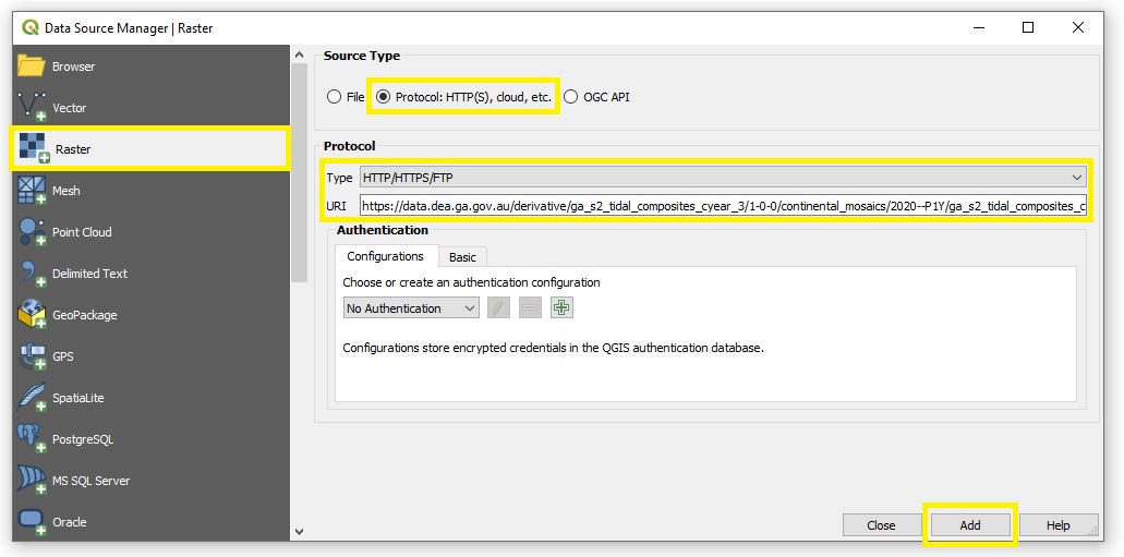
.tiffiles representing a particular band e.g.ga_s2ls_intertidal_cyear_3_2018_elevation.tif> click Copy link address.In QGIS, click Layer > Add Layer > Add Raster Layer.
For Source Type, select Protocol: HTTP(S), cloud, etc..
For Protocol Type, select HTTP/HTTPS/FTP.
In the URI field, paste the link to the band that you copied to the clipboard.
Click Add to start streaming the layer. Data should appear on the map after a few seconds (or after several minutes on slow internet connections).
Learn more about streaming cloud datasets: How to read a Cloud Optimized GeoTIFF with QGIS.
Stream continental COG mosaics in Esri ArcGIS Pro
To connect Esri ArcGIS Pro to DEA’s Amazon S3 bucket, follow Esri’s tutorial: Create a cloud storage connection.
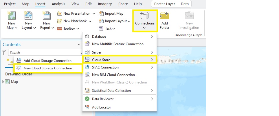
In ArcGIS Pro, click the Insert tab, then click Connections > Cloud Store > New Cloud Storage Connection.
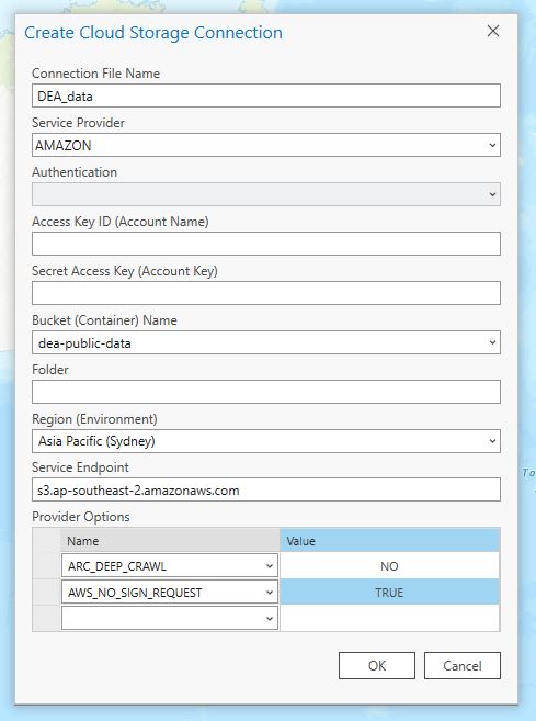
Add the following details to the Create Cloud Storage Connection dialogue box:
Connection File Name —
DEA_dataService Provider —
AMAZONBucket Name (Container) —
dea-public-dataRegion (Environment) —
Asia Pacific (Sydney)Service Endpoint —
s3.ap-southeast-2.amazonaws.comProvider Options
ARC_DEEP_CRAWL—NOAWS_NO_SIGN_REQUEST—TRUE
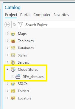
In the Catalog pane:
Expand Cloud Stores.
Expand the DEA_data.acs cloud store.
Navigate to
derivative/ga_s2ls_intertidal_cyear_3/2-0-0/continental_mosaics/.Enter a directory of a particular year, e.g.
2018--P1Y.Drag and drop the
.tifCOG file representing a particular band e.g.ga_s2ls_intertidal_cyear_3_2018_elevation.tifonto the map (or right-click and “Add to map”).
Important
When adding COG files to ArcGIS Pro, select No when asked whether to build statistics for the layer.
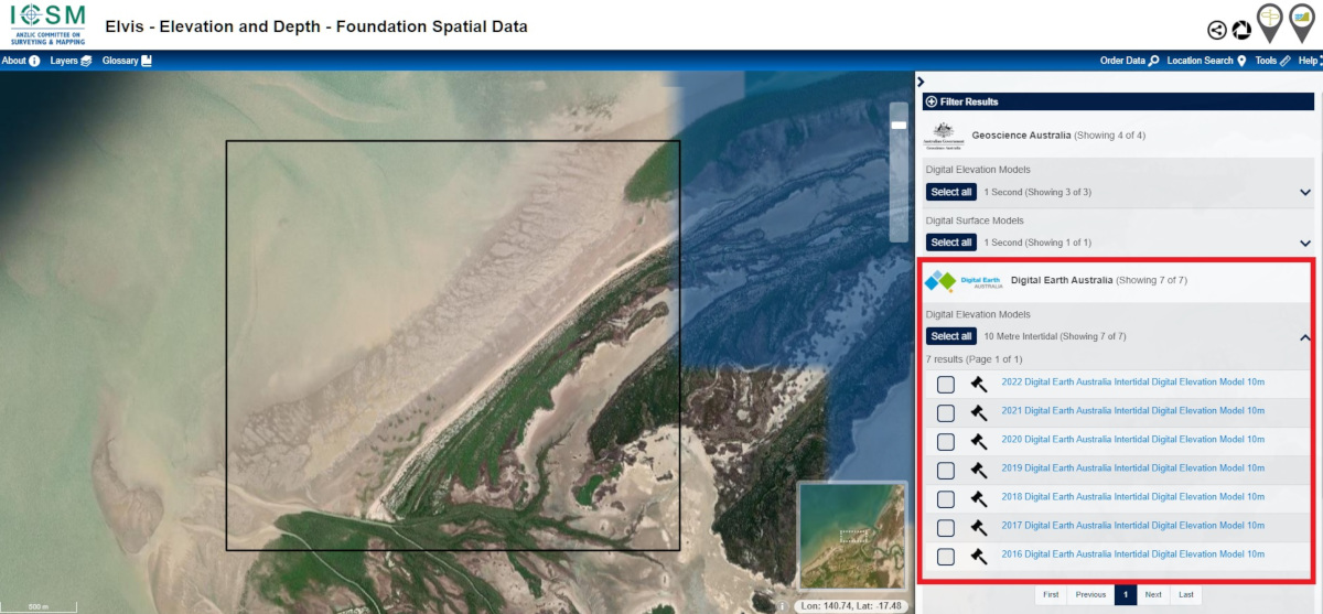
How to download data from ELVIS
To download the data from the ELVIS (Elevation Information System) platform, follow these steps.
Open the ELVIS platform.
Zoom in to your coastal area of interest on the ELVIS map.
Click Order data on the top-right of the page.
Select your desired selection method, then click Draw.
Select your area of interest on the map, then click Search.
In the Search Results menu (on the right side), locate the 10 Metre Intertidal DEM results and select the years of data you wish to order.
Enter your industry and email address, then click Order dataset.
Your data will be emailed to you as a zipped folder containing DEA Intertidal Elevation and Elevation Uncertainty GeoTIFF rasters.
How to download data from individual tiles (Not recommended)
Warning
Downloading individual tiles is not recommended, but can be useful for accessing small amounts of data.
Open the DEA Intertidal directory in DEA’s Amazon S3 bucket.
Click on
ga_summary_grid_c3_32km_coastal.geojsonto download the file to your computer. This file can be used in a GIS package to identify the product tiles that you require for a given location. (Alternatively, you can access this file via DEA Maps to identify the required tiles: Sea, ocean and coast > DEA Intertidal > DEA Intertidal 32 km tile grid.)Open the DEA Intertidal directory in DEA’s Amazon S3 bucket and navigate into the folder of the tile that you require. The folder names are based on the ‘x’ and ‘y’ coordinate references. E.g. first enter the
x082folder, then they122.Enter a directory of a particular year, e.g.
2018--P1YClick to download the product layer of interest, e.g.
ga_s2ls_intertidal_cyear_3_x082y122_2021--P1Y_final_extents.tif. Learn more about file naming and product layers: Technical Information.
Version history
Versions are numbered using the Semantic Versioning scheme (Major.Minor.Patch). Note that this list may include name changes and predecessor products.
v2.0.0 |
- |
Current version |
v1.0.0 |
of |
|
v2.0.0 |
of |
|
v1.0.0 |
of |
Changelog
DEA Intertidal 2.0.0
In May 2025, DEA Intertidal was updated to version 2.0.0 and 2023 data was added to all layers in the product suite. This update also includes the following changes.
The DEA Intertidal Extents layer was added. This new data layer, in combination with the existing elevation and exposure layers supersedes the DEA Intertidal Extents Model (ITEM) product. (The ITEM product has hence been deprecated.)
Ensemble tide modelling is now delivered via the eo-tides tide modelling Python package.
New quality assessment layers were added: qa_count_clear and qa_coastal_connectivity.
DEA Intertidal 1.0.0
In April 2024, version 1.0.0 was released of the DEA Intertidal product suite. The elevation data layer of this product supersedes the National Intertidal Digital Elevation Model product. (The Intertidal Elevation product has hence been deprecated.)
Acknowledgments
The authors would like to sincerely thank the following individuals and organisations for validation data and valuable feedback on preliminary versions of this product.
Mick O’Leary/Ryan Lowe — University of Western Australia
Jenna Hounslow/Adrian Gleiss — Murdoch University
Mitchell Baum — University of Melbourne
Lucya Roncevich — Western Australia Department of Transport
Duncan Moore — GA Maritime Jurisdiction Advice
Ben Ford — Department of Climate Change, Energy, Environment and Water
Maria Zann — QLD Department of Environment and Science
Rob Beaman — James Cook University
Kathy Murray — WA Department of Biodiversity, Conservation and Attractions
Hannah Power — University of Newcastle
Mitch Lyons — University of New South Wales
Nick Murray — James Cook University
Airborne Research Australia
Northern Territory Government
License and copyright
© Commonwealth of Australia (Geoscience Australia).
Released under Creative Commons Attribution 4.0 International Licence.