DEA Maps
DEA Maps is an online platform where you can view Digital Earth Australia (DEA) datasets. It aims to make it easy for anyone to access our open-source data — whether you are a scientist, educator, journalist, or otherwise.
Quick links
Open DEA Maps to get started.
Filter by location if you don’t see any data or data doesn’t cover a location.
Add data to the map
Let’s add a dataset to the map so that we can view the data. Here’s an example map of the DEA Surface Reflectance (Sentinel-2A MSI) dataset.
Open DEA Maps.
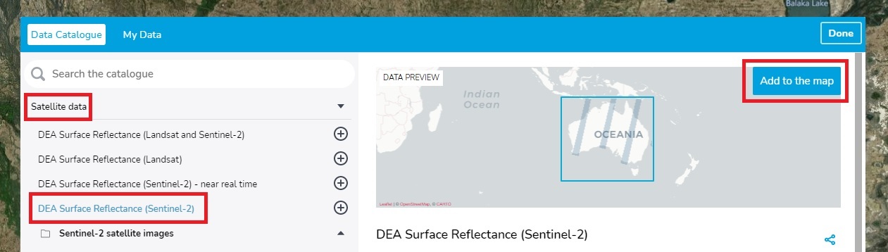
Click Explore map data.
In the data catalogue, navigate through the folders to find the dataset that you want to access then add it to the map. E.g. click Baseline satellite data > DEA Surface Reflectance (Sentinel-2) > DEA Surface Reflectance (Sentinel-2A MSI) > Add to the map.
The dataset will be added as a card to the left sidebar and you may now see data overlaid on the map. But if you don’t see any data or data doesn’t cover a location, continue to the next section: Filter by location.
Filter by location
After adding data to the map, if you don’t see any data or the data doesn’t cover a particular location, you can use the ‘Filter by location’ tool. This is especially useful for datasets that are provided as swaths (strips of data that the satellite captures as it travels), e.g. the ‘Baseline satellite data’ datasets. Zoom out on the map and you will often see that swaths of data are visible, but they are not covering the location you are interested in. Or you may find that no data exists at all for this particular time.
‘Filter by location’ will show the most recent data that is available for a given location.
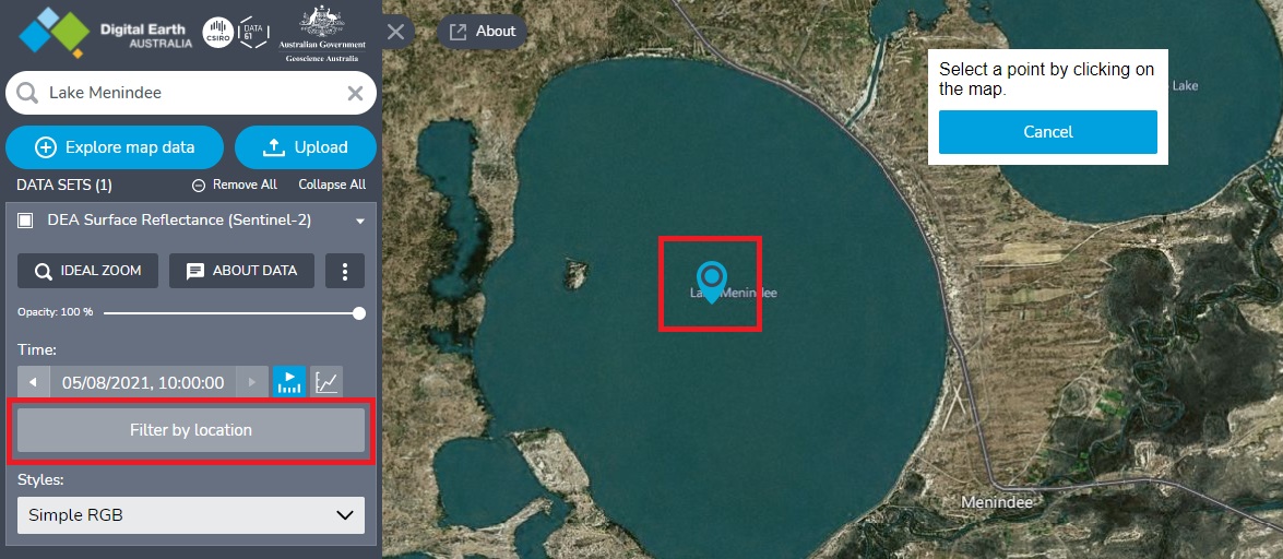
In the left sidebar, click Filter by location for the dataset you have added the map.
Click a location on the map then wait for it to load.
Data should now be overlaid on that location. The left sidebar will indicate that the filter has been applied.
Next, you can either select Remove filter or New location.
Share a URL and save your map
Once you’ve created a map by adding datasets, adjusting map settings, and zooming in on a specific location, you will want to share this map with others, or save it so you can come back to it later. You can do both of these using the ‘Share URL’ feature.
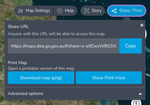
Click Share / Print on the top right.
Click Copy to copy this custom URL to your clipboard.
Anyone who opens this URL will see the map with the same configurations and viewing location. You can send this URL to others, link to it from a public website, or bookmark it for later.
Switch styles (bands and layers)
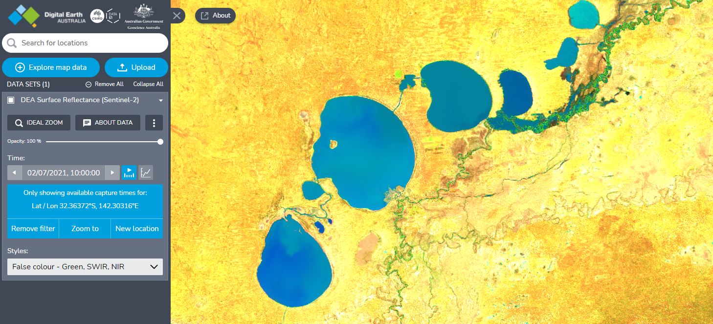
Most datasets contain multiple ‘bands’ or ‘layers’ of data that reveal different features of the landscape. You can switch between these using the Styles dropdown in the left sidebar.
For example, the ‘DEA Surface Reflectance (Sentinel-2)’ dataset can be switched to the ‘False colour - Green, SWIR, NIR’ style. This style uses wavelengths of light beyond the visible spectrum (‘near infrared’ and ‘short-wave infrared’) to highlight waterbodies, vegetation, and other features more distinctly.
Compare side-by-side
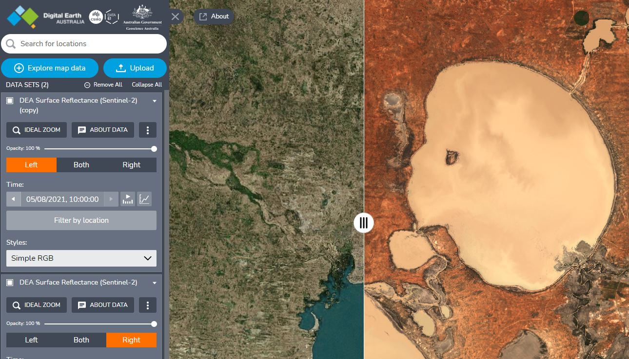
There is a Compare feature that lets you view two different map configurations side-by-side. This allows you to compare two different datasets or the same dataset at two different times. Here’s an example map of DEA High Tide Imagery versus DEA Low Tide Imagery.
In the left sidebar, click the
 button (‘Show more actions’) on a dataset that you have added to the map > click Compare.
The map will now be split into two halves. In the sidebar, the dataset’s card will be split into two separate cards: one labelled ‘Left’ and the other ‘Right’.
You can drag the divider to easily see the difference between the two sides.
You can configure each side of the map independently. E.g. you can change the ‘Styles’ value on the right side.
Each dataset can be assigned to either the Left or Right side or Both by selecting the relevant option in the left sidebar.
To compare two different datasets side-by-side: add an additional dataset to the map > assign it to the right or left side > remove the existing dataset that was assigned to that side.
To close this side-by-side view, click the “×” next to ‘Split Screen Mode’ in the left sidebar.
Note that you can share a URL of your comparison by using the Share / Print feature.
Difference tool
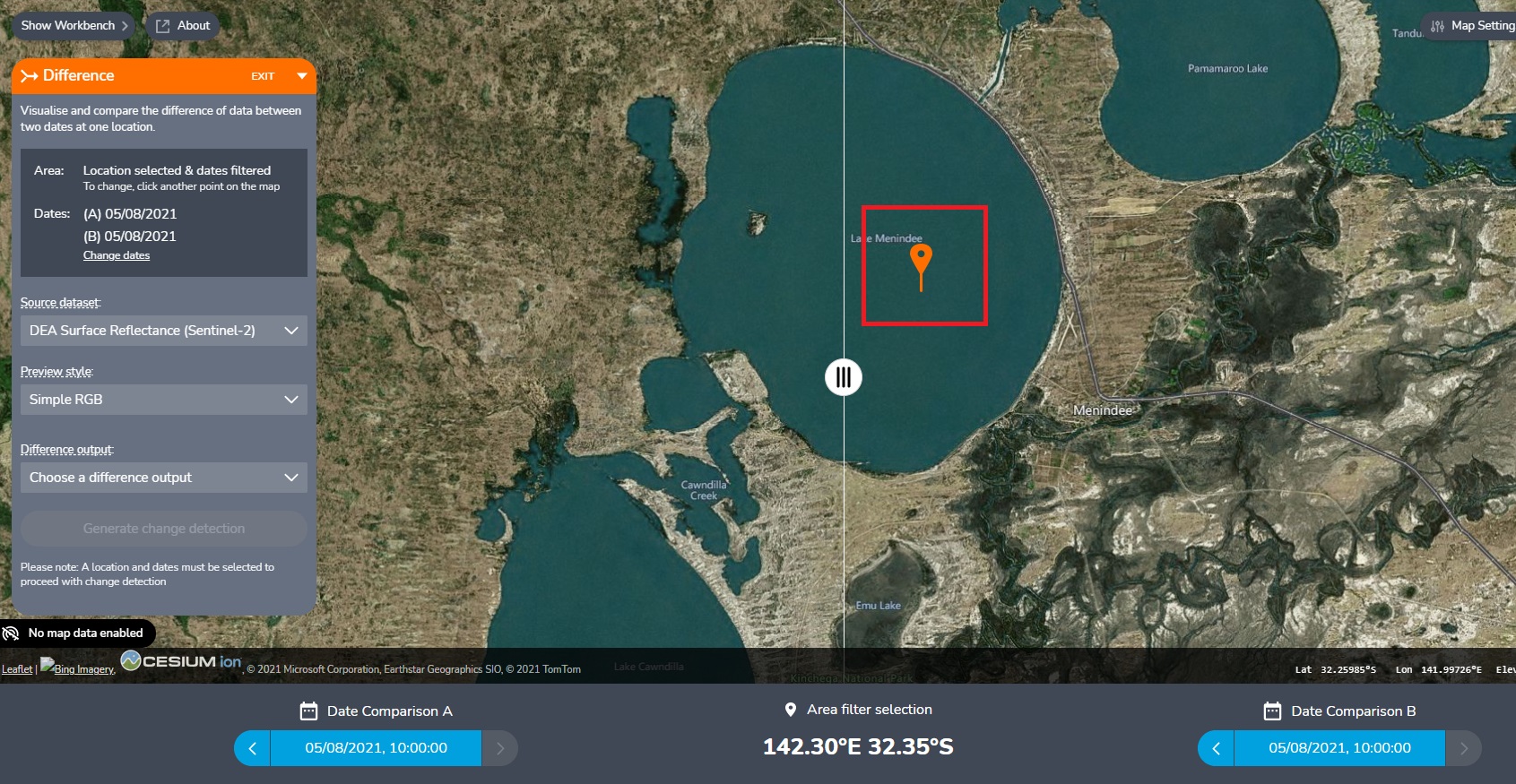
The Difference tool allows you to visualise the changes in a dataset over time. Here is an example map showing locations that have gotten wetter or dryer over time.
In the left sidebar, click the
button (‘Show more actions’) on a dataset that you have added to the map > click Difference.The difference tool will appear, replacing the left sidebar.
Select a location on the map to analyse by clicking anywhere on the map.
Under Data Comparison A and Date Comparison B, choose the two dates to compare. For best results, choose dates that don’t have cloud cover.
Click Choose a difference output and select an option. For instance, the ‘Modified Normalised Difference Water Index - Green, SWIR’ is useful for comparing the distribution of water.
Click Generate change detection.
The difference will be shown on the map as a new dataset. For instance, the ‘Modified Normalised Difference Water Index - Green, SWIR’ shows locations that have gotten wetter over time in blue while locations that have gotten dryer are red.
To reopen the left sidebar, click Show workbench, and to close the difference tool, click Exit. You’ll notice that in the left sidebar, the difference has been added as a dataset.
Export data as high-resolution TIFF
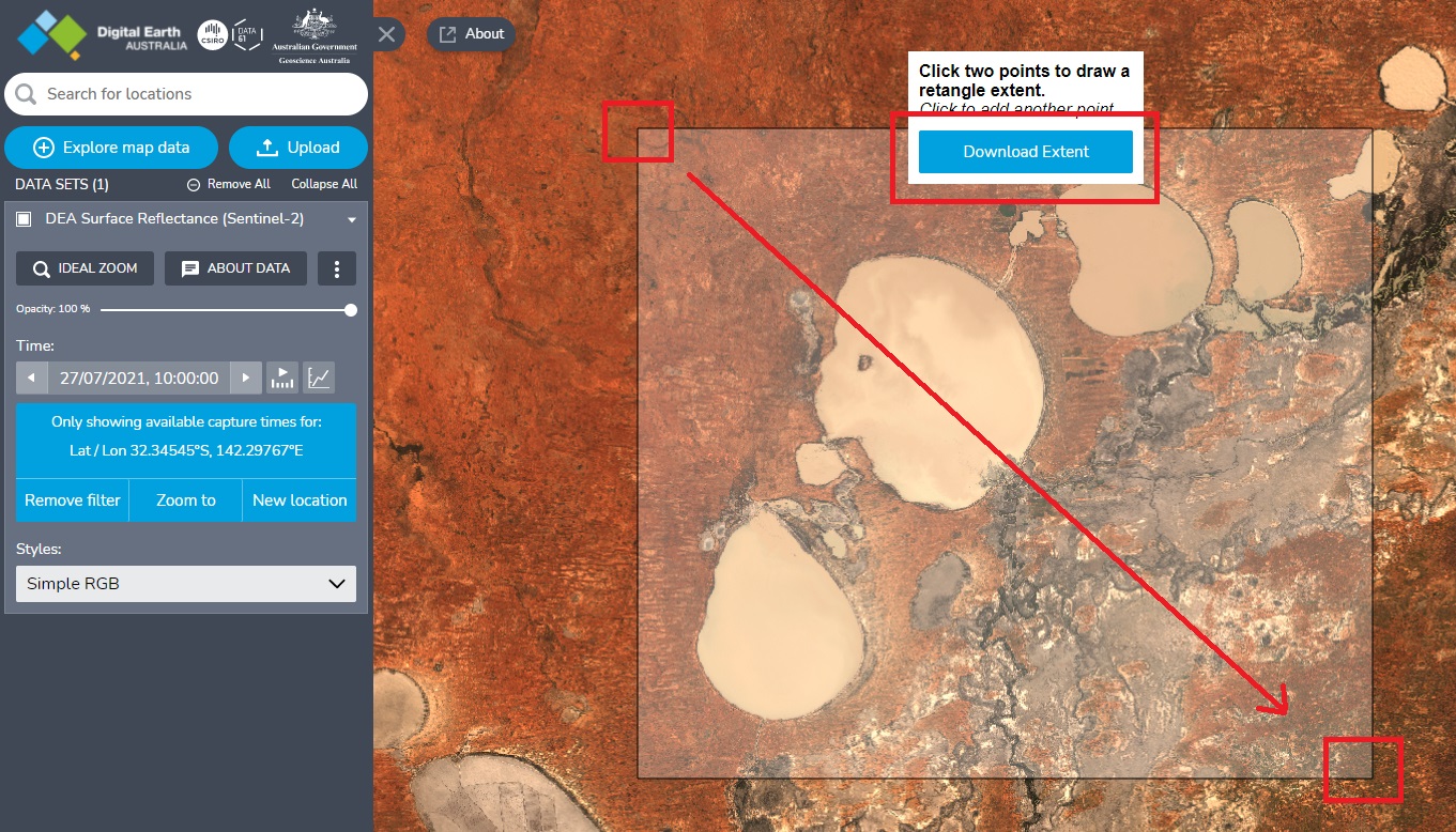
It’s possible to export small areas of DEA data in the high-resolution TIFF image format. This exported data can used in GIS applications like QGIS and ArcGIS. (But for exporting larger volumes of data, you can use the DEA Sandbox or NCI environments or download directly from the DEA Public Data S3 Bucket.)
In the left sidebar, click the
button (‘Show more actions’) on a dataset that you have added to the map > click Export.Click two locations on the map to draw a rectangle.
Click Download extent then wait for the TIFF file to be downloaded to your computer. (If the export fails, try zooming in and drawing a rectangle that covers a smaller land area.)
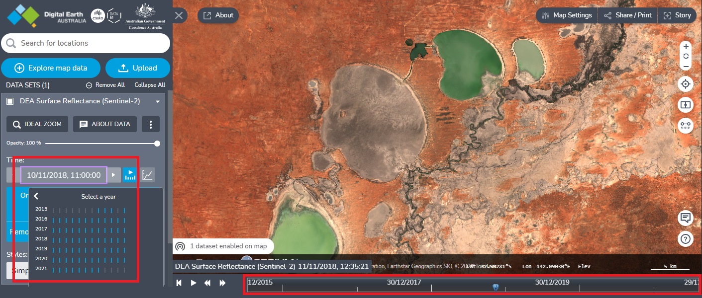
Navigate time and location
You can navigate through datasets across a range of times and locations.
Change to a different time by clicking the Time value in the left sidebar, or clicking on the timeline at the bottom.
Zoom in and out of the map by scrolling the mouse, or use the “+” and “-” buttons.
Move to a different location by dragging with the mouse, or use the Search for locations bar. E.g. search for ‘Lake Eyre’, then click ‘Lake Eyre, SA’ to jump straight to this location.
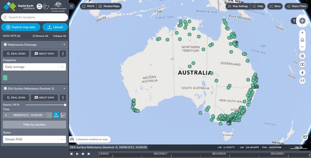
Watercourse Discharge
The Bureau of Meteorology provides water discharge data for 3,500 hydrological measurement stations across Australia. DEA’s Water Discharge tool allows you to plot watercourse discharge information on a map and match it to the relevant satellite images for a particular date.
Add a dataset to your map, e.g. ‘DEA Surface Reflectance (Sentinel-2A MSI)’.
Add the Watercourse Discharge dataset to your map: Explore map data > Other > Water Regulations Data (BoM) > Hydrologic Reference Stations > Watercourse Discharge > Add to the map. The Hydrological Reference Stations will be plotted on the map. These are the locations where watercourse discharge is measured by the Bureau of Meteorology.
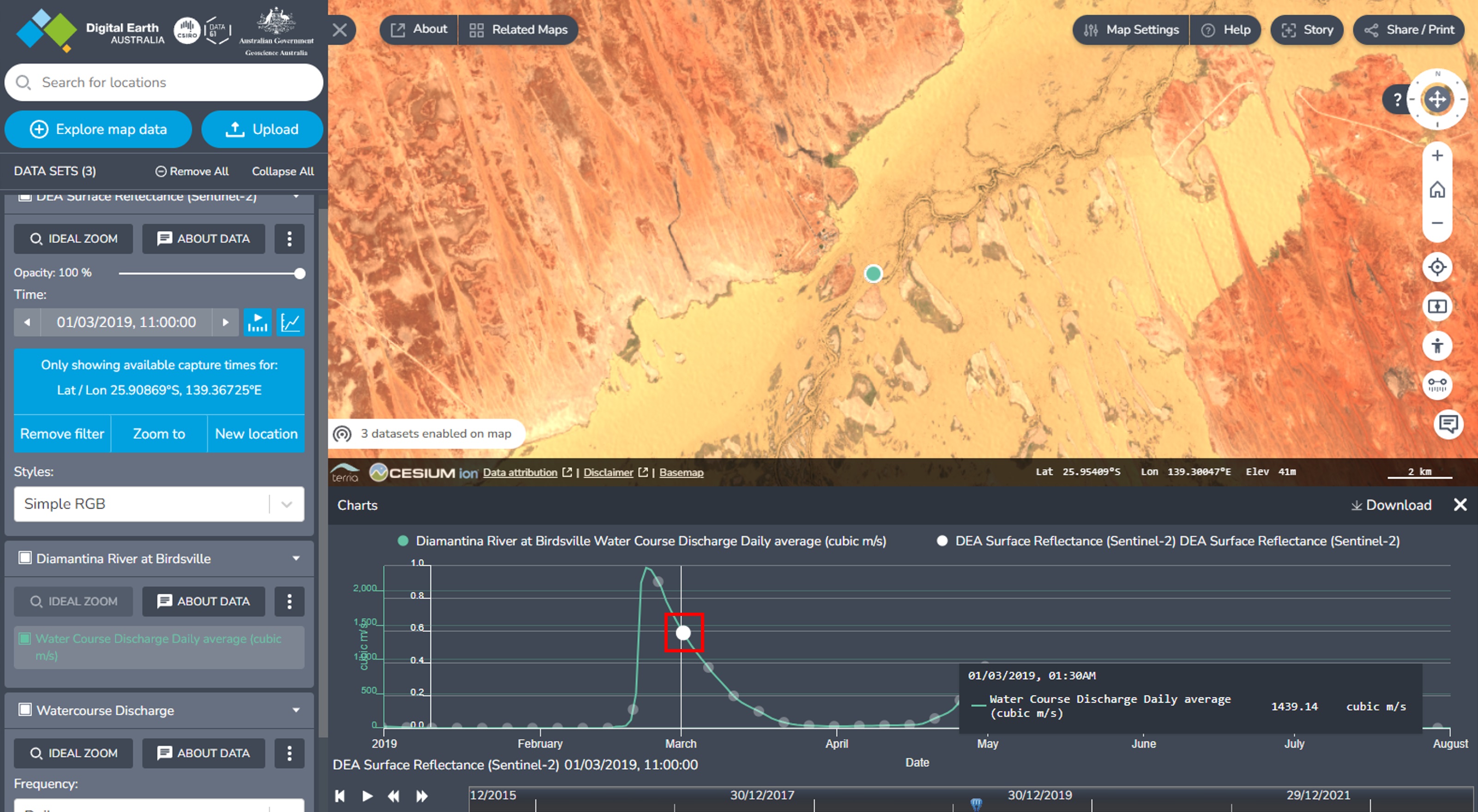
Zoom in and click on one of these stations. A ‘Feature Information’ popup will provide details about the station.
In the popup, click Show <dataset> at this location, e.g. ‘Show DEA Surface Reflectance (Sentinel-2A MSI) at this location’.
In the popup, click Expand to expand the hydrograph of this particular station, then click × to close the popup. You can hover your mouse over the hydrograph to view the average watercourse discharge value for each date.
To add your chosen dataset to the hydrograph, in the left sidebar, on the dataset’s card, click the
 button (‘Show available times on chart’).
Each capture in your chosen dataset will display as a dot on the hydrograph. To view the dots more clearly, you can zoom in on the hydrograph by scrolling your mouse. Click on a dot to jump to the particular time and location of the capture on the map.
Other useful features
Print your map — Click Share / Print > Show Print View > a new page will open showing a printer-friendly view; click Print or press Ctrl-p on your keyboard.
Capture a high-quality image of your map — Follow the steps above to print your map, except on the printer-friendly page, right-click on the image and select Save image as.
Animate satellite imagery — Once you have added a dataset to the map, click the ‘Play’ button on the timeline at the bottom. You can adjust the speed using the ‘Play faster’ and ‘Play slower’ buttons.
Dataset documentation — To learn more about a dataset and how to use its specific features on the map, see its Data Product page. For example, the DEA Waterbodies (Landsat) page explains how to view information about waterbodies and compare waterbodies on the map.
Learn more — To learn more about using DEA Maps, click Help on the top right, then you can take the tour, watch the videos, or read the guides.