Detecting change in urban extent 
Sign up to the DEA Sandbox to run this notebook interactively from a browser
Compatibility: Notebook currently compatible with both the
NCIandDEA SandboxenvironmentsProducts used: ga_ls8c_ard_3
Background
The rate at which cities and towns grow, or the urbanisation rate, is an important indicator of the sustainability of towns and cities. Rapid, unplanned urbanisation can result in poor social, economic, and environmental outcomes due to inadequate and overburdened infrastructure and services creating congestion, worsening air pollution, and leading to a shortage of adequate housing.
The first requirement for addressing the impacts of rapid urbanisation is to accurately and regularly monitor urban expansion in order to track urban development over time. Earth Observation datasets, such as those available through the Digital Earth Australia platform provide a cost-effective and accurate means of mapping the urban extent of cities.
Description
This notebook conducts the following analysis:
Load Landsat 8 data over the city/region of interest
Generate geomedian composites for the baseline and more recent year.
Calculate the Enhanced Normalised Difference Impervious Surfaces Index (ENDISI)
Threshold the ENDISI plots to delineate urban extent
Compare the urban extent in the baseline year to the more recent urban extent
Getting started
To run this analysis, run all the cells in the notebook, starting with the “Load packages” cell.
Load packages
Import Python packages that are used for the analysis.
[1]:
%matplotlib inline

import datacube
import numpy as np
import xarray as xr
import matplotlib.pyplot as plt
from odc.algo import xr_geomedian
from matplotlib.patches import Patch
from matplotlib.colors import ListedColormap

import sys
sys.path.insert(1, '../Tools/')
from dea_tools.datahandling import load_ard
from dea_tools.plotting import rgb, display_map
from dea_tools.bandindices import calculate_indices
from dea_tools.dask import create_local_dask_cluster
/env/lib/python3.8/site-packages/geopandas/_compat.py:106: UserWarning: The Shapely GEOS version (3.8.0-CAPI-1.13.1 ) is incompatible with the GEOS version PyGEOS was compiled with (3.9.1-CAPI-1.14.2). Conversions between both will be slow.
  warnings.warn(
Set up a Dask cluster
Dask can be used to better manage memory use down and conduct the analysis in parallel. For an introduction to using Dask with Digital Earth Australia, see the Dask notebook.
Note: We recommend opening the Dask processing window to view the different computations that are being executed; to do this, see the Dask dashboard in DEA section of the Dask notebook.
To use Dask, set up the local computing cluster using the cell below.
[2]:
create_local_dask_cluster()
Client
|
Cluster
|
Connect to the datacube
Activate the datacube database, which provides functionality for loading and displaying stored Earth observation data.
[3]:
dc = datacube.Datacube(app='Urban_change_detection')
Analysis parameters
The following cell set important parameters for the analysis:
lat: The central latitude to analyse (e.g.-35.1836).lon: The central longitude to analyse (e.g.149.1210).buffer: The number of square degrees to load around the central latitude and longitude. For reasonable loading times, set this as0.1or lower.baseline_year: The baseline year, to use as the baseline of urbanisation (e.g.2014)analysis_year: The analysis year to analyse the change in urbanisation (e.g.2019)
[4]:
# Alter the lat and lon to suit your study area
lat, lon = -35.1836, 149.1210
# Provide your area of extent here
buffer = 0.05

# Combine central lat,lon with buffer to get area of interest
lat_range = (lat - buffer, lat + buffer)
lon_range = (lon - buffer, lon + buffer)

# Change the years values also here
# Note: Landsat 8 starts from 2013
baseline_year = 2014
analysis_year = 2020
View the selected location
The next cell will display the selected area on an interactive map. Feel free to zoom in and out to get a better understanding of the area you’ll be analysing. Clicking on any point of the map will reveal the latitude and longitude coordinates of that point.
[5]:
display_map(lon_range, lat_range)
[5]:
Load cloud-masked Landsat-8 data
The first step in this analysis is to load in Landsat data for the lat_range, lon_range and time_range we provided above.
The code below uses the load_ard function to load in data from the Landsat 8 satellite for the area and time specified. For more information, see the Using load_ard notebook. The function will also automatically mask out clouds from the dataset, allowing us to focus on pixels that contain useful data:
[6]:
# Create a query
query = {
    'time': (f'{baseline_year}', f'{analysis_year}'),
    'x': lon_range,
    'y': lat_range,
    'resolution': (-30, 30),
    'measurements': ['swir1', 'swir2', 'blue', 'green', 'red'],
    'group_by': 'solar_day',
}

# Create a dataset of the requested data
ds = load_ard(dc=dc,
              products=['ga_ls8c_ard_3'],
              output_crs='EPSG:3577',
              dask_chunks={'time': 1, 'x': 2000, 'y': 2000},
              **query)
Finding datasets
    ga_ls8c_ard_3
Applying pixel quality/cloud mask
Returning 316 time steps as a dask array
Calculate the geomedian for each year
Here we group the timeseries into years and calculate the geomedian (geometric median) for each year.
Note: For more information about computing geomedians, see the Generating Geomedian Composites notebook.
[7]:
# Group by year, then calculate the geomedian on each year
geomedians = ds.groupby('time.year').map(xr_geomedian)
geomedians
[7]:
<xarray.Dataset>
Dimensions:  (x: 351, y: 409, year: 7)
Coordinates:
  * y        (y) float64 -3.941e+06 -3.941e+06 ... -3.953e+06 -3.953e+06
  * x        (x) float64 1.546e+06 1.546e+06 1.546e+06 ... 1.556e+06 1.556e+06
  * year     (year) int64 2014 2015 2016 2017 2018 2019 2020
Data variables:
    swir1    (year, y, x) float32 dask.array<chunksize=(1, 409, 351), meta=np.ndarray>
    swir2    (year, y, x) float32 dask.array<chunksize=(1, 409, 351), meta=np.ndarray>
    blue     (year, y, x) float32 dask.array<chunksize=(1, 409, 351), meta=np.ndarray>
    green    (year, y, x) float32 dask.array<chunksize=(1, 409, 351), meta=np.ndarray>
red (year, y, x) float32 dask.array<chunksize=(1, 409, 351), meta=np.ndarray>- x: 351
- y: 409
- year: 7
- y(y)float64-3.941e+06 ... -3.953e+06
- units :
- metre
- resolution :
- -30.0
- crs :
- EPSG:3577
array([-3940515., -3940545., -3940575., ..., -3952695., -3952725., -3952755.])
- x(x)float641.546e+06 1.546e+06 ... 1.556e+06
- units :
- metre
- resolution :
- 30.0
- crs :
- EPSG:3577
array([1545945., 1545975., 1546005., ..., 1556385., 1556415., 1556445.])
- year(year)int642014 2015 2016 2017 2018 2019 2020
array([2014, 2015, 2016, 2017, 2018, 2019, 2020])
- swir1(year, y, x)float32dask.array<chunksize=(1, 409, 351), meta=np.ndarray>
- units :
- 1
- crs :
- EPSG:3577
- grid_mapping :
- spatial_ref
Array Chunk Bytes 4.02 MB 574.24 kB Shape (7, 409, 351) (1, 409, 351) Count 10621 Tasks 7 Chunks Type float32 numpy.ndarray - swir2(year, y, x)float32dask.array<chunksize=(1, 409, 351), meta=np.ndarray>
- units :
- 1
- crs :
- EPSG:3577
- grid_mapping :
- spatial_ref
Array Chunk Bytes 4.02 MB 574.24 kB Shape (7, 409, 351) (1, 409, 351) Count 10621 Tasks 7 Chunks Type float32 numpy.ndarray - blue(year, y, x)float32dask.array<chunksize=(1, 409, 351), meta=np.ndarray>
- units :
- 1
- crs :
- EPSG:3577
- grid_mapping :
- spatial_ref
Array Chunk Bytes 4.02 MB 574.24 kB Shape (7, 409, 351) (1, 409, 351) Count 10621 Tasks 7 Chunks Type float32 numpy.ndarray - green(year, y, x)float32dask.array<chunksize=(1, 409, 351), meta=np.ndarray>
- units :
- 1
- crs :
- EPSG:3577
- grid_mapping :
- spatial_ref
Array Chunk Bytes 4.02 MB 574.24 kB Shape (7, 409, 351) (1, 409, 351) Count 10621 Tasks 7 Chunks Type float32 numpy.ndarray - red(year, y, x)float32dask.array<chunksize=(1, 409, 351), meta=np.ndarray>
- units :
- 1
- crs :
- EPSG:3577
- grid_mapping :
- spatial_ref
Array Chunk Bytes 4.02 MB 574.24 kB Shape (7, 409, 351) (1, 409, 351) Count 10621 Tasks 7 Chunks Type float32 numpy.ndarray
time dimension has been replaced by the year dimension. Since the query was for all data between our target years, we have data for all years in the range.Note: As we are using
dask, no data reading or calculations have yet taken place.
[8]:
geomedians = geomedians.sel(year=[baseline_year, analysis_year])
geomedians
[8]:
<xarray.Dataset>
Dimensions:  (x: 351, y: 409, year: 2)
Coordinates:
  * y        (y) float64 -3.941e+06 -3.941e+06 ... -3.953e+06 -3.953e+06
  * x        (x) float64 1.546e+06 1.546e+06 1.546e+06 ... 1.556e+06 1.556e+06
  * year     (year) int64 2014 2020
Data variables:
    swir1    (year, y, x) float32 dask.array<chunksize=(1, 409, 351), meta=np.ndarray>
    swir2    (year, y, x) float32 dask.array<chunksize=(1, 409, 351), meta=np.ndarray>
    blue     (year, y, x) float32 dask.array<chunksize=(1, 409, 351), meta=np.ndarray>
    green    (year, y, x) float32 dask.array<chunksize=(1, 409, 351), meta=np.ndarray>
red (year, y, x) float32 dask.array<chunksize=(1, 409, 351), meta=np.ndarray>- x: 351
- y: 409
- year: 2
- y(y)float64-3.941e+06 ... -3.953e+06
- units :
- metre
- resolution :
- -30.0
- crs :
- EPSG:3577
array([-3940515., -3940545., -3940575., ..., -3952695., -3952725., -3952755.])
- x(x)float641.546e+06 1.546e+06 ... 1.556e+06
- units :
- metre
- resolution :
- 30.0
- crs :
- EPSG:3577
array([1545945., 1545975., 1546005., ..., 1556385., 1556415., 1556445.])
- year(year)int642014 2020
array([2014, 2020])
- swir1(year, y, x)float32dask.array<chunksize=(1, 409, 351), meta=np.ndarray>
- units :
- 1
- crs :
- EPSG:3577
- grid_mapping :
- spatial_ref
Array Chunk Bytes 1.15 MB 574.24 kB Shape (2, 409, 351) (1, 409, 351) Count 10623 Tasks 2 Chunks Type float32 numpy.ndarray - swir2(year, y, x)float32dask.array<chunksize=(1, 409, 351), meta=np.ndarray>
- units :
- 1
- crs :
- EPSG:3577
- grid_mapping :
- spatial_ref
Array Chunk Bytes 1.15 MB 574.24 kB Shape (2, 409, 351) (1, 409, 351) Count 10623 Tasks 2 Chunks Type float32 numpy.ndarray - blue(year, y, x)float32dask.array<chunksize=(1, 409, 351), meta=np.ndarray>
- units :
- 1
- crs :
- EPSG:3577
- grid_mapping :
- spatial_ref
Array Chunk Bytes 1.15 MB 574.24 kB Shape (2, 409, 351) (1, 409, 351) Count 10623 Tasks 2 Chunks Type float32 numpy.ndarray - green(year, y, x)float32dask.array<chunksize=(1, 409, 351), meta=np.ndarray>
- units :
- 1
- crs :
- EPSG:3577
- grid_mapping :
- spatial_ref
Array Chunk Bytes 1.15 MB 574.24 kB Shape (2, 409, 351) (1, 409, 351) Count 10623 Tasks 2 Chunks Type float32 numpy.ndarray - red(year, y, x)float32dask.array<chunksize=(1, 409, 351), meta=np.ndarray>
- units :
- 1
- crs :
- EPSG:3577
- grid_mapping :
- spatial_ref
Array Chunk Bytes 1.15 MB 574.24 kB Shape (2, 409, 351) (1, 409, 351) Count 10623 Tasks 2 Chunks Type float32 numpy.ndarray
Load the data and calculate the geomedian for the selected years
Now that we have the geomedians for the two years we want to analyse, we can trigger the delay-loading and calculation.
This will use the dask cluster we set up earlier. You can follow the progress of this step by opening the Dask processing window. See the Dask dashboard in DEA section of the Dask notebook.
Note: This step can take several minutes to complete.
[9]:
%%time
geomedians = geomedians.compute()
CPU times: user 3.76 s, sys: 402 ms, total: 4.16 s
Wall time: 3min 9s
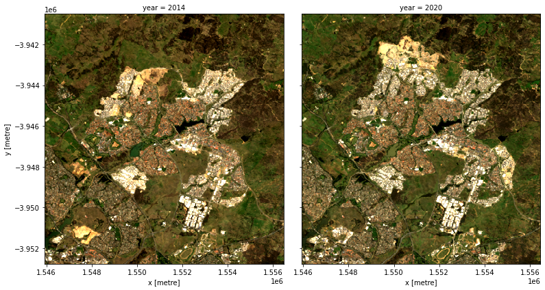
View the satellite data
We can plot the two years to visually compare them:
[10]:
rgb(geomedians, bands=['red', 'green', 'blue'], col='year')
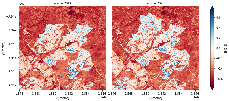
Calculate ENDISI
The Enhanced Normalized Difference Impervious Surfaces Index (ENDISI) is a recently developed urbanisation proxy that has been shown to work well in a variety of environments (Chen et al. 2020). Like all normalised difference indicies, it has a range of [-1, 1]. Note that MNDWI, swir_diff and alpha are all part of the ENDISI calculation.
[11]:
def MNDWI(dataset):
    return calculate_indices(dataset, index='MNDWI', collection='ga_ls_3').MNDWI


def swir_diff(dataset):
    return dataset.swir1 / dataset.swir2


def alpha(dataset):
    return (2 * (np.mean(dataset.blue))) / (np.mean(swir_diff(dataset)) +
                                            np.mean(MNDWI(dataset)**2))


def ENDISI(dataset):
    mndwi = MNDWI(dataset)
    swir_diff_ds = swir_diff(dataset)
    alpha_ds = alpha(dataset)
    return (dataset.blue - (alpha_ds) *
            (swir_diff_ds + mndwi**2)) / (dataset.blue + (alpha_ds) *
                                       (swir_diff_ds + mndwi**2))
[12]:
# Calculate the ENDISI index
geomedians['ENDISI'] = ENDISI(geomedians)
Let’s plot the ENDISI images so we can see if the urban areas are distinguishable
[13]:
geomedians.ENDISI.plot(col='year',
                       vmin=-.75,
                       vmax=0.75,
                       cmap='RdBu',
                       figsize=(12, 5),
                       robust=True);
And now plot the histogram of all the pixels in the ENDISI array:
[14]:
geomedians.ENDISI.plot.hist(bins=1000,
                            range=(-1, 1),
                            facecolor='gray',
                            figsize=(10, 4))
plt.title('ENDISI Histogram');
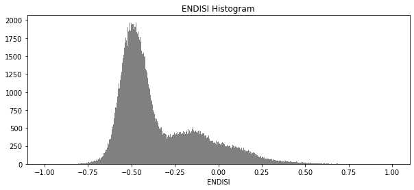
Calculate urban extent
To define the urban extent, we need to threshold the ENDISI arrays. Values above this threshold will be labelled as ‘Urban’ while values below the trhehsold will be excluded from the urban extent. We can determine this threshold a number of ways (inluding by simply manually definining it e.g. threshold=-0.1). Below, we use the Otsu method to automatically threshold the image.
[15]:
from skimage.filters import threshold_otsu

threshold = threshold_otsu(geomedians.ENDISI.values)
print(round(threshold, 2))
-0.25
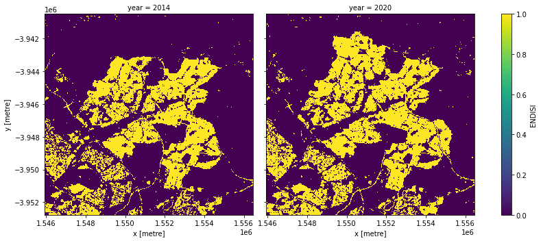
Apply the threshold
We apply the threshold and plot both years side-by-side.
[16]:
urban_area = (geomedians.ENDISI > threshold).astype(int)
urban_area.plot(
    col='year',
    figsize=(12, 5),
    robust=True
);
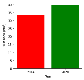
Plotting the change in urban extent
We can convert the data above into a total area for each year, then plot a bar graph.
[17]:
pixel_length = query["resolution"][1]  # in metres
area_per_pixel = pixel_length**2 / 1000**2

# Calculate urban area in square kilometres
urban_area_km2 = urban_area.sum(dim=['x', 'y']) * area_per_pixel

# Plot the resulting area through time
fig, axes = plt.subplots(1, 1, figsize=(4, 4))
plt.bar([0, 1],
        urban_area_km2,
        tick_label=urban_area_km2.year,
        width=0.8,
        color=['red', 'green'])
axes.set_xlabel("Year")
axes.set_ylabel("Built area (km$^2$)")
print('Urban extent in ' + str(baseline_year) + ': ' +
      str(urban_area_km2.sel(year=baseline_year).values) + ' km2')
print('Urban extent in ' + str(analysis_year) + ': ' +
      str(urban_area_km2.sel(year=analysis_year).values) + ' km2')
Urban extent in 2014: 33.641999999999996 km2
Urban extent in 2020: 39.7296 km2
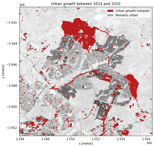
Urban growth hotspots
If we subtract the ENDISI of the baseline year from the analysis year, we can highlight regions where urban growth is occurring. To ensure we aren’t capturing all change, we can set a change threshold, beyond which we distinguish between real change from background variation.
In this plot, we can see areas that have seen significant change, highlighting regions of urbanisation.
[18]:
change_threshold = 0.15
[19]:
# Calculate the change in BU between the years
urban_change = geomedians.ENDISI.sel(
    year=analysis_year) - geomedians.ENDISI.sel(year=baseline_year)

# Plot urban extent from first year in grey as a background
baseline_urban = xr.where(urban_area.sel(year=baseline_year), 1, np.nan)
plot = geomedians.ENDISI.sel(year=baseline_year).plot(cmap='Greys',
                                                      size=8,
                                                      aspect=urban_area.y.size /
                                                      urban_area.y.size,
                                                      add_colorbar=False)

# Plot the meaningful change in urban area
to_urban = '#b91e1e'
xr.where(urban_change > change_threshold, 1,
         np.nan).plot(ax=plot.axes,
                      add_colorbar=False,
                      cmap=ListedColormap([to_urban]))

# Add the legend
plot.axes.legend([Patch(facecolor=to_urban),
                  Patch(facecolor='darkgrey'),
                  Patch(facecolor='white')],
                 ['Urban growth hotspots', 'Remains urban'])
plt.title('Urban growth between ' + str(baseline_year) + ' and ' +
          str(analysis_year));
Next steps
When you are done, return to the Analysis parameters section, modify some values (e.g. lat, lon or time) and rerun the analysis.
You can use the interactive map in the View the selected location section to find new central latitude and longitude values by panning and zooming, and then clicking on the area you wish to extract location values for. You can also use Google maps to search for a location you know, then return the latitude and longitude values by clicking the map.
Additional information
License: The code in this notebook is licensed under the Apache License, Version 2.0. Digital Earth Australia data is licensed under the Creative Commons by Attribution 4.0 license.
Contact: If you need assistance, please post a question on the Open Data Cube Discord chat or on the GIS Stack Exchange using the open-data-cube tag (you can view previously asked questions here). If you would like to report an issue with this notebook, you can file one on
GitHub.
Last modified: December 2023
Compatible datacube version:
[20]:
print(datacube.__version__)
1.8.5