Identifying shipping lanes with radar 
Sign up to the DEA Sandbox to run this notebook interactively from a browser
Compatibility: Notebook currently compatible with the
DEA Sandboxenvironment onlyProducts used: s1_gamma0_geotif_scene
Background
Being able to spot ships and shipping lanes from satellite imagery can be useful for gaining a holistic picture of maritime traffic. The properties of radar data can be utilised to detect where ships appear over time, highlighting the presence of shipping lanes.
When working with radar data, water commonly appears dark; its relatively smooth surface results in very little backscatter, and consequently, low intensities are recorded by the satellite in both polarisation bands. However, if a large ship is on the water, the backscatter at the ship’s location will be much higher than the water.
This notebook was inspired by this thread on Twitter.
Sentinel-1 use case
The ESA/EC Copernicus Sentinel-1 mission has been operating since April 2014. The two satellites (Sentinel-1A and 1B) have a frequent revisit time of 6 days. This helps to build a large catalogue of observations that can be leveraged to identify shipping lanes.
Description
In this example, we attempt to identify shipping lanes around Australia by taking advantage of the fact that ships on the water result in a large radar backscatter signal. This can be done by finding the maximum of each pixel in Sentinel-1 images. Computing the maximum value for many pixels is computationally expensive, so we make use of the parallel-computing library Dask. The worked example takes user through the code required to
Load Sentinel-1 backscatter data for an area of interest.
Calculate the maximum value for each pixel using Dask.
Visualise the maximum values to identify shipping lanes.
Getting started
To run this analysis, run all the cells in the notebook, starting with the “Load packages” cell.
After finishing the analysis, return to the “Analysis parameters” cell, modify some values (e.g. choose a different location or time period to analyse) and re-run the analysis. There are additional instructions on modifying the notebook at the end.
Load packages
Load key Python packages and supporting functions for the analysis.
[1]:
%matplotlib inline

import dask
import datacube
import numpy as np
import matplotlib.pyplot as plt
from dask.distributed import Client

import sys
sys.path.insert(1, '../Tools/')
from dea_tools.dask import create_local_dask_cluster
from dea_tools.plotting import display_map
Connect to the datacube
Activate the datacube database, which provides functionality for loading and displaying stored Earth observation data.
[2]:
dc = datacube.Datacube(app="Shipping_lane_identification")
Set up distributed computing
Calculating the maximum value for each pixel in an image can be computationally expensive. However, it is possible to reduce the computation time by parallelising the process through Dask. Access to Dask is provided as part of the DEA environment.
To set up distributed computing with Dask, you need to first set up a Dask client using the function below:
Note: For more information about using Dask, refer to the Parallel processing with Dask notebook.
[3]:
create_local_dask_cluster()
/usr/local/lib/python3.6/dist-packages/distributed/dashboard/core.py:79: UserWarning:
Port 8787 is already in use.
Perhaps you already have a cluster running?
Hosting the diagnostics dashboard on a random port instead.
  warnings.warn("\n" + msg)
Client
|
Cluster
|
Analysis parameters
The following cell sets the parameters, which define the area of interest and the length of time to conduct the analysis over. The parameters are
latitude: The latitude range to analyse (e.g.(-41.277, -40.977)). For reasonable loading times, make sure the range spans less than ~0.1 degrees.longitude: The longitude range to analyse (e.g.(146.145, 146.545)). For reasonable loading times, make sure the range spans less than ~0.1 degrees.time: The date range to analyse (e.g.('2017-01-01', '2018-01-01')).
If running the notebook for the first time, keep the default settings below. This will demonstrate how the analysis works and provide meaningful results. The example covers Devonport, Tasmania, which is where the Spirit of Tasmania (the ferry between Melbourne and Tasmania) transits from.
To run the notebook for a different area, make sure Sentinel-1 data is available for the chosen area using the DEA Explorer. We provide a list of additional ports to try at the end of this notebook.
[4]:
# Define the area of interest
latitude = (-41.277, -40.977)
longitude = (146.145, 146.545)

# Set the range of dates for the analysis
time = ("2017-01-01", "2018-01-01")
View the selected location
The next cell will display the selected area on an interactive map. Feel free to zoom in and out to get a better understanding of the area you’ll be analysing. Clicking on any point of the map will reveal the latitude and longitude coordinates of that point.
[5]:
display_map(x=longitude, y=latitude)
/usr/local/lib/python3.6/dist-packages/pyproj/crs.py:77: FutureWarning: '+init=<authority>:<code>' syntax is deprecated. '<authority>:<code>' is the preferred initialization method.
  return _prepare_from_string(" ".join(pjargs))
/usr/local/lib/python3.6/dist-packages/pyproj/crs.py:77: FutureWarning: '+init=<authority>:<code>' syntax is deprecated. '<authority>:<code>' is the preferred initialization method.
  return _prepare_from_string(" ".join(pjargs))
[5]:
Load and view Sentinel-1 data
The first step in the analysis is to load Sentinel-1 backscatter data for the specified area of interest. As part of specifying the load, the dask_chunks argument is used to tell Dask how to segement the data for parallelised computations (see the xarray documentation).
[6]:
ds = dc.load(
    product="s1_gamma0_geotif_scene",
    x=longitude,
    y=latitude,
    output_crs="epsg:3577",
    resolution=(-25, 25),
    time=time,
    dask_chunks={"x": 4000, "y": 4000, "time": 1}
)

ds
<xarray.Dataset>
Dimensions:  (time: 115, x: 1511, y: 1452)
Coordinates:
  * time     (time) datetime64[ns] 2017-01-01T19:25:41.446675 ... 2017-12-27T19:26:13.739366
  * y        (y) float64 -4.548e+06 -4.548e+06 ... -4.584e+06 -4.584e+06
  * x        (x) float64 1.209e+06 1.209e+06 1.209e+06 ... 1.246e+06 1.246e+06
Data variables:
    vh       (time, y, x) float32 dask.array<chunksize=(1, 1452, 1511), meta=np.ndarray>
    vv       (time, y, x) float32 dask.array<chunksize=(1, 1452, 1511), meta=np.ndarray>
Attributes:
    crs:      epsg:3577
Visualise loaded data
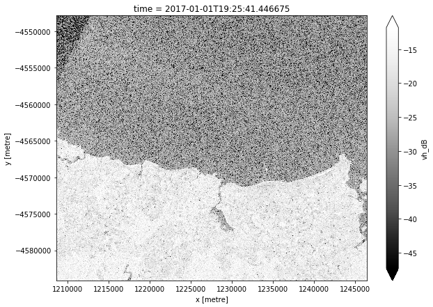
Sentinel-1 backscatter data has two measurements, VV and VH, which correspond to the polarisation of the light sent and received by the satellite. VV refers to the satellite sending out vertically-polarised light and receiving vertically-polarised light back, whereas VH refers to the satellite sending out vertically-polarised light and receiving horizontally-polarised light back. These two measurement bands can tell us different information about the area we’re studying.
When working with radar backscatter, it is common to work with the data in units of decibels (dB), rather than digital number (DN) as measured by the satellite. To convert from DN to dB, we use the following formula:
The code below visualises the VH band for the first timestep in the dataset:
[7]:
# Scale to plot data in decibels
ds["vh_dB"] = 10 * np.log10(ds.vh)

# Plot all VH observations for the year
ds.vh_dB.isel(time=0).plot(cmap="Greys_r", robust=True, figsize=(10,7))
plt.show()
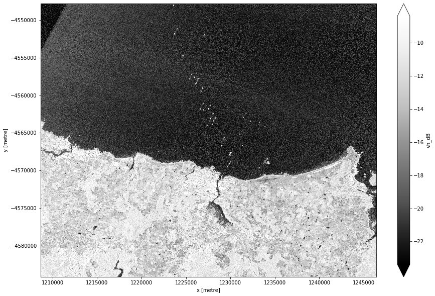
Calculating and plotting the maximum pixel value
After loading the data, we can calculate the maximum value for each pixel measured in decibels. Note that the Dask operation will occur when attempting to plot the vh_dB band in the cell below.
[8]:
max_vh = ds.vh_dB.max(dim="time")

max_vh.plot.imshow(size=10, cmap="Greys_r", robust=True)
plt.show()
Conclusion
The high contrast between the ships and the water can make for striking images. Fortunately, processing with Dask makes it possible to make these computationally-intensive images in under a minute, even for very large areas.
Only a year of data is available at the moment, but more observations would likely lead to clearer identification of the shipping lanes.
Next steps
When you are done, return to the “Set up analysis” cell, modify some values (e.g. latitude and longitude) and rerun the analysis.
There are a number of key ports covered by DEA Sentinel-1 data. The available data can be viewed on the DEA Explorer, but we also list the latitude and longitude coordinates for a few key ports below.
New South Wales
Port of Newcastle
This is one of Australia’s largest ports, with a diverse range of cargo types.
latitude = (-33.128, -32.728)
longitude = (151.582, 151.982)
Port Kembla
This is the home to New South Wales’ largest motor vehicle import hub and grain export terminal.
latitude = (-34.685, -34.285)
longitude = (150.699, 151.099)
Port Jackson
This includes Sydney Harbour, which houses numerous cruise ships and ferries.
latitude = (-34.046, -33.646)
longitude = (151.049, 151.449)
Northern Territory
Port Darwin
This is a key port in Darwin, covering livestock, containers, and cruise ships.
latitude = (-12.617, -12.217)
longitude = (130.600, 131.000)
Additional information
License: The code in this notebook is licensed under the Apache License, Version 2.0. Digital Earth Australia data is licensed under the Creative Commons by Attribution 4.0 license.
Contact: If you need assistance, please post a question on the Open Data Cube Discord chat or on the GIS Stack Exchange using the open-data-cube tag (you can view previously asked questions here). If you would like to report an issue with this notebook, you can file one on
GitHub.
Last modified: December 2023
Compatible datacube version:
[ ]:
print(datacube.__version__)
Tags
Tags: sandbox compatible, NCI compatible, sentinel 1, display_map, real world, water, radar, maritime, image compositing, Dask, parallel processing