Exporting cloud-optimised GeoTIFF files 
Sign up to the DEA Sandbox to run this notebook interactively from a browser
Compatibility: Notebook currently compatible with both the
NCIandDEA SandboxenvironmentsProducts used: ga_ls8c_ard_3
Background
At the end of an analysis it can be useful to export data to a GeoTIFF file (e.g. outputname.tif), either to save results or to allow for exploring results in a GIS software platform (e.g. ArcGIS or QGIS).
A Cloud Optimized GeoTIFF (COG) is a regular GeoTIFF file (i.e. that can be opened by GIS software like QGIS or ArcMap) aimed at being hosted on a HTTP file server, with an internal organization that enables more efficient workflows on the cloud.
Description
This notebook shows a number of ways to export a GeoTIFF file using the datacube.utils.cog function write_cog:
Exporting a single-band, single time-slice GeoTIFF from an xarray object loaded through a
dc.loadqueryExporting a multi-band, single time-slice GeoTIFF from an xarray object loaded through a
dc.loadqueryExporting multiple GeoTIFFs, one for each time-slice of an xarray object loaded through a
dc.loadquery
In addition, the notebook demonstrates several more advanced applications of write_cog: 1. Exporting data from lazily loaded dask arrays 2. Passing in custom rasterio parameters to override the function’s defaults
Getting started
To run this analysis, run all the cells in the notebook, starting with the “Load packages” cell.
Load packages
[1]:
import rasterio
import datacube
from datacube.utils.cog import write_cog

import sys
sys.path.insert(1, '../Tools/')
from dea_tools.plotting import rgb
Connect to the datacube
[2]:
dc = datacube.Datacube(app='Exporting_GeoTIFFs')
Load Landsat 8 data from the datacube
Here we are loading in a timeseries of Landsat 8 satellite images through the datacube API. This will provide us with some data to work with.
[3]:
# Create a query object
query = {
    'x': (149.06, 149.17),
    'y': (-35.27, -35.32),
    'time': ('2020-01', '2020-03'),
    'measurements': ['nbart_red', 'nbart_green', 'nbart_blue'],
    'output_crs': 'EPSG:3577',
    'resolution': (-30, 30),
    'group_by': 'solar_day'
}

# Load available data from the Landsat 8
ds = dc.load(product='ga_ls8c_ard_3', **query)

# Print output data
ds
[3]:
<xarray.Dataset>
Dimensions:      (time: 11, y: 229, x: 356)
Coordinates:
  * time         (time) datetime64[ns] 2020-01-07T23:56:40.592891 ... 2020-03...
  * y            (y) float64 -3.955e+06 -3.955e+06 ... -3.962e+06 -3.962e+06
  * x            (x) float64 1.544e+06 1.544e+06 ... 1.554e+06 1.554e+06
    spatial_ref  int32 3577
Data variables:
    nbart_red    (time, y, x) int16 1691 1729 1738 1734 1695 ... 799 799 819 753
    nbart_green  (time, y, x) int16 1380 1386 1405 1398 1377 ... 879 911 877 808
    nbart_blue   (time, y, x) int16 1170 1168 1175 1171 1156 ... 670 670 685 642
Attributes:
    crs:           EPSG:3577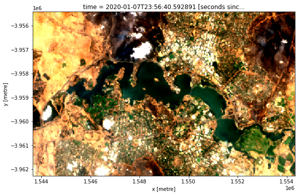
grid_mapping: spatial_refPlot an rgb image to confirm we have data
The white regions are cloud cover.
[4]:
rgb(ds, index=0, percentile_stretch=(0.1, 0.9))
Export GeoTIFFs
Single-band, single time-slice data
This method uses the datacube.utils.cog function write_cog (where COG stands for Cloud Optimised GeoTIFF) to export a simple single-band, single time-slice GeoTIFF file. A few important caveats should be noted when using this function:
It requires an
xarray.DataArray; supplying anxarray.Datasetwill return an error. To convert anxarray.Datasetto anxarray.DataArrayrun the following:
da = ds.to_array()
This function generates a temporary in-memory GeoTIFF file without compression. This means the function will temporarily use about 1.5 to 2 times the memory of the input
xarray.DataArray
[5]:
# Select a single time-slice and a single band from the dataset.
singleband_da = ds.nbart_red.isel(time=0)

# Write GeoTIFF to a location
write_cog(geo_im=singleband_da,
          fname='red_band.tif',
          overwrite=True)
[5]:
PosixPath('red_band.tif')
Multi-band, single time-slice data
Here we select a single time and export all the bands in the dataset using write_cog:
[6]:
# Select a single time-slice
rgb_da = ds.isel(time=0).to_array()

# Write multi-band GeoTIFF to a location
write_cog(geo_im=rgb_da,
          fname='rgb.tif',
          overwrite=True)
[6]:
PosixPath('rgb.tif')
Multi-band, multiple time-slice data
If we want to export all of the time steps in a dataset, we can wrap write_cog in a for-loop and export each time slice as an individual GeoTIFF file:
[7]:
for i in range(len(ds.time)):

    # We will use the date of the satellite image to name the GeoTIFF
    date = ds.isel(time=i).time.dt.strftime('%Y-%m-%d').data
    print(f'Writing {date}')

    # Convert current time step into a `xarray.DataArray`
    singletimestamp_da = ds.isel(time=i).to_array()

    # Write GeoTIFF
    write_cog(geo_im=singletimestamp_da,
              fname=f'{date}.tif',
              overwrite=True)
Writing 2020-01-07
Writing 2020-01-16
Writing 2020-01-23
Writing 2020-02-01
Writing 2020-02-08
Writing 2020-02-17
Writing 2020-02-24
Writing 2020-03-04
Writing 2020-03-11
Writing 2020-03-20
Writing 2020-03-27
Exporting GeoTIFFs from a dask array
Note: For more information on using
dask, refer to the Parallel processing with Dask notebook
If you pass a lazily-loaded dask array into the function, write_cog will not immediately output a GeoTIFF, but will instead return a dask.delayed object:
[8]:
# Lazily load data using dask
ds_dask = dc.load(product='ga_ls8c_ard_3',
                  dask_chunks={},
                  **query)

# Run `write_cog`
ds_delayed = write_cog(geo_im=ds_dask.isel(time=0).to_array(),
                       fname='dask_geotiff.tif',
                       overwrite=True)

# Print dask.delayed object
print(ds_delayed)
Delayed('_write_cog-94418718-68c7-4e80-a786-c75e7d6fe50a')
To trigger the GeoTIFF to be exported to file, run .compute() on the dask.delayed object. The file will now appear in the file browser to the left.
[9]:
ds_delayed.compute()
[9]:
PosixPath('dask_geotiff.tif')
Advanced
Passing custom rasterio parameters
By default, write_cog will read attributes like nodata directly from the attributes of the data itself. However, write_cog also accepts any parameters that could be passed to the underlying `rasterio.open <https://rasterio.readthedocs.io/en/latest/api/rasterio.io.html>`__ function, so these can be used to override the default attribute values.
For example, it can be useful to provide a new nodata value, for instance if data is transformed to a different dtype or scale and the original nodata value is no longer appropriate. By default, write_cog will use a nodata value of -999 as this is what is stored in the dataset’s attributes:
[10]:
# Select a single time-slice and a single band from the dataset.
singleband_da = ds.nbart_red.isel(time=0)

# Print nodata attribute value
print(singleband_da.nodata)
-999
To override this value and use a nodata value of 0 instead:
[11]:
# Write GeoTIFF
write_cog(geo_im=singleband_da,
          fname='custom_nodata.tif',
          overwrite=True,
          nodata=0.0)
[11]:
PosixPath('custom_nodata.tif')
We can verify the nodata value is now set to 0.0 by reading the data back in with rasterio:
[12]:
with rasterio.open('custom_nodata.tif') as geotiff:
    print(geotiff.nodata)
0.0
Unsetting nodata for float datatypes containing NaN
A common analysis workflow is to load data from the datacube, then mask out certain values by setting them to NaN. For example, we may use the .where() method to set all -999 nodata values in our data to NaN:
Note: The
mask_invalid_datafunction fromdatacube.utils.maskingcan also be used to automatically setnodatavalues from the data’s attributes toNaN. This function will also automatically drop thenodataattribute from the data, removing the need for the steps below. For more information, see the Masking data notebook.
[13]:
# Select a single time-slice and a single band from the dataset.
singleband_da = ds.nbart_red.isel(time=0)

# Set -999 values to NaN
singleband_masked = singleband_da.where(singleband_da != -999)
singleband_masked
[13]:
<xarray.DataArray 'nbart_red' (y: 229, x: 356)>
array([[1691., 1729., 1738., ..., 1180., 1347., 1175.],
       [1680., 1731., 1763., ..., 1140., 1220., 1158.],
       [1737., 1778., 1816., ..., 1070., 1047., 1131.],
       ...,
       [1766., 1808., 1830., ..., 1175., 1069., 1050.],
       [1748., 1731., 1687., ..., 1423., 1193., 1119.],
       [1520., 1802., 1868., ..., 1417., 1340., 1296.]])
Coordinates:
    time         datetime64[ns] 2020-01-07T23:56:40.592891
  * y            (y) float64 -3.955e+06 -3.955e+06 ... -3.962e+06 -3.962e+06
  * x            (x) float64 1.544e+06 1.544e+06 ... 1.554e+06 1.554e+06
    spatial_ref  int32 3577
Attributes:
    units:         1
    nodata:        -999
    crs:           EPSG:3577
grid_mapping: spatial_refIn this case, since we have replaced -999 nodata values with NaN, the data’s nodata attribute is no longer valid. Before we write our data to file, we should therefore remove the nodata attribute from our data:
[14]:
# Remove nodata attribute
singleband_masked.attrs.pop('nodata')

# Write GeoTIFF
write_cog(geo_im=singleband_masked,
          fname='masked_data.tif',
          overwrite=True)
[14]:
PosixPath('masked_data.tif')
If we read this GeoTIFF back in with rasterio, we will see that it no longer has a nodata attribute set:
[15]:
with rasterio.open('masked_data.tif') as geotiff:
    print(geotiff.nodata)
None
Additional information
License: The code in this notebook is licensed under the Apache License, Version 2.0. Digital Earth Australia data is licensed under the Creative Commons by Attribution 4.0 license.
Contact: If you need assistance, please post a question on the Open Data Cube Discord chat or on the GIS Stack Exchange using the open-data-cube tag (you can view previously asked questions here). If you would like to report an issue with this notebook, you can file one on
GitHub.
Last modified: December 2023
Compatible datacube version:
[16]:
print(datacube.__version__)
1.8.6
Tags
Tags: sandbox compatible, NCI compatible, GeoTIFF, Cloud Optimised GeoTIFF, dc.load, landsat 8, datacube.utils.cog, write_cog, exporting data