Introduction to DEA Fractional Cover

• Sign up to the DEA Sandbox to run this notebook interactively from a browser

• Compatibility: Notebook currently compatible with both the NCI and DEA Sandbox environments

• Products used: ga_ls_fc_3, ga_ls_wo_3

Background

Fractional cover data can be used to identify large scale patterns and trends and inform evidence based decision making and policy on topics including wind and water erosion risk, soil carbon dynamics, land management practices and rangeland condition.

This information is used by policy agencies, natural and agricultural land resource managers, and scientists to monitor land conditions over large areas over long time frames.

What this product offers

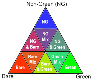
Fractional Cover (FC), developed by the Joint Remote Sensing Research Program, is a measurement that splits the landscape into three parts, or fractions:

• green (leaves, grass, and growing crops)

• brown (branches, dry grass or hay, and dead leaf litter)

• bare ground (soil or rock)

DEA uses Fractional Cover to characterise every 30 m square of Australia for any point in time from 1987 to today.

Applications

Fractional cover provides valuable information for a range of environmental and agricultural applications, including:

• soil erosion monitoring

• land surface process modelling

• land management practices (e.g. crop rotation, stubble management, rangeland management)

• vegetation studies

• fuel load estimation

• ecosystem modelling

• land cover mapping

Note: For more technical information about DEA Fractional Cover, visit the official Geoscience Australia DEA Fractional Cover product description.

Description

This notebook will demonstrate how to load DEA Fractional Cover using Digital Earth Australia. Topics covered include:

1. Inspecting the products and measurements available in the datacube

2. Loading DEA Fractional Cover for an example location

3. Plotting fractional cover as false colour images

4. Inspecting unmixing error outputs

5. Masking out missing or invalid data and unclear or wet pixels, and using this to track percentages of green and brown vegetation and bare soil over time

---

Getting started

To run this analysis, run all the cells in the notebook, starting with the “Load packages” cell.

Load packages

Import Python packages that are used for the analysis.

import datacube
from datacube.utils import masking
import matplotlib.pyplot as plt

import sys
sys.path.insert(1, '../Tools/')
from dea_tools.datahandling import wofs_fuser
from dea_tools.plotting import rgb, plot_wo

Connect to the datacube

Connect to the datacube so we can access DEA data.

dc = datacube.Datacube(app='DEA_Fractional_Cover')

/env/lib/python3.8/site-packages/datacube/drivers/postgres/_api.py:48: RemovedIn20Warning: Deprecated API features detected! These feature(s) are not compatible with SQLAlchemy 2.0. To prevent incompatible upgrades prior to updating applications, ensure requirements files are pinned to "sqlalchemy<2.0". Set environment variable SQLALCHEMY_WARN_20=1 to show all deprecation warnings.  Set environment variable SQLALCHEMY_SILENCE_UBER_WARNING=1 to silence this message. (Background on SQLAlchemy 2.0 at: https://sqlalche.me/e/b8d9)
  select([

Available products and measurements

List products available in Digital Earth Australia

We can use datacube’s list_products functionality to inspect DEA Fractional Cover products that are available in Digital Earth Australia. The table below shows the product name that we will use to load data, and a brief description of the product.

# List DEA Fractional Cover products available in DEA
dc_products = dc.list_products()
dc_products.loc[['ga_ls_fc_3']]

	name	description	license	default_crs	default_resolution
name
ga_ls_fc_3	ga_ls_fc_3	Geoscience Australia Landsat Fractional Cover ...	CC-BY-4.0	EPSG:3577	(-30, 30)

List measurements

We can inspect the contents of the DEA Fractional Cover product using datacube’s list_measurements functionality. The table below lists each of the measurements available in the product, which represent unique data variables that provide information about the vegetation and bare soil cover in each pixel:

• pv: The fractional cover of green vegetation

• npv: The fractional cover of non-green vegetation

• bs: The fractional cover of bare soil

• ue: The fractional cover unmixing error

The table also provides information about the measurement data types, units, nodata value and other technical information about each measurement.

dc_measurements = dc.list_measurements()
dc_measurements.loc[['ga_ls_fc_3']]

		name	dtype	units	nodata	aliases	flags_definition	spectral_definition
product	measurement
ga_ls_fc_3	bs	bs	uint8	percent	255	[bare]	NaN	NaN
	pv	pv	uint8	percent	255	[green_veg]	NaN	NaN
	npv	npv	uint8	percent	255	[dead_veg]	NaN	NaN
	ue	ue	uint8	1	255	[err]	NaN	NaN

Loading data

Now that we know what products and measurements are available for the products, we can load data from Digital Earth Australia for an example location:

# Set up a region to load data
query = {
    'y': (-34.06813, -34.22099),
    'x': (139.83315, 140.05151),
    'time': ('1993-10-15', '1993-11-20'),
}

# Load DEA Fractional Cover data from the datacube
fc = dc.load(product='ga_ls_fc_3',
             measurements=['bs', 'pv', 'npv', 'ue'],
             output_crs='EPSG:32754',
             resolution=(-30, 30),
             group_by='solar_day',
             **query)

We can now view the data that we loaded. The measurements listed under Data variables should match the measurements displayed in the previous List measurements step.

fc

<xarray.Dataset>
Dimensions:      (time: 4, y: 573, x: 678)
Coordinates:
  * time         (time) datetime64[ns] 1993-10-21T23:55:41.593257 ... 1993-11...
  * y            (y) float64 6.23e+06 6.23e+06 6.23e+06 ... 6.213e+06 6.213e+06
  * x            (x) float64 3.923e+05 3.924e+05 ... 4.126e+05 4.126e+05
    spatial_ref  int32 32754
Data variables:
    bs           (time, y, x) uint8 16 19 16 24 20 29 33 ... 17 20 16 23 26 13
    pv           (time, y, x) uint8 51 52 53 52 50 38 26 ... 32 28 30 26 20 31
    npv          (time, y, x) uint8 32 27 29 23 29 32 40 ... 50 51 53 50 53 55
    ue           (time, y, x) uint8 13 13 12 12 11 9 9 ... 13 12 12 13 11 11 13
Attributes:
    crs:           EPSG:32754
    grid_mapping:  spatial_ref

xarray.Dataset

• Dimensions:
  • time: 4
  • y: 573
  • x: 678
• Coordinates: (4)
  • time
    (time)
    datetime64[ns]
    1993-10-21T23:55:41.593257 ... 1...

    units :

    seconds since 1970-01-01 00:00:00

    array(['1993-10-21T23:55:41.593257000', '1993-10-30T23:49:28.344073000',
           '1993-11-06T23:55:11.515323000', '1993-11-15T23:49:18.275417000'],
          dtype='datetime64[ns]')

  • y
    (y)
    float64
    6.23e+06 6.23e+06 ... 6.213e+06

    units :

    metre

    resolution :

    -30.0

    crs :

    EPSG:32754

    array([6229875., 6229845., 6229815., ..., 6212775., 6212745., 6212715.])

  • x
    (x)
    float64
    3.923e+05 3.924e+05 ... 4.126e+05

    units :

    metre

    resolution :

    30.0

    crs :

    EPSG:32754

    array([392325., 392355., 392385., ..., 412575., 412605., 412635.])

  • spatial_ref
    ()
    int32
    32754

    spatial_ref :

    PROJCS["WGS 84 / UTM zone 54S",GEOGCS["WGS 84",DATUM["WGS_1984",SPHEROID["WGS 84",6378137,298.257223563,AUTHORITY["EPSG","7030"]],AUTHORITY["EPSG","6326"]],PRIMEM["Greenwich",0,AUTHORITY["EPSG","8901"]],UNIT["degree",0.0174532925199433,AUTHORITY["EPSG","9122"]],AUTHORITY["EPSG","4326"]],PROJECTION["Transverse_Mercator"],PARAMETER["latitude_of_origin",0],PARAMETER["central_meridian",141],PARAMETER["scale_factor",0.9996],PARAMETER["false_easting",500000],PARAMETER["false_northing",10000000],UNIT["metre",1,AUTHORITY["EPSG","9001"]],AXIS["Easting",EAST],AXIS["Northing",NORTH],AUTHORITY["EPSG","32754"]]

    grid_mapping_name :

    transverse_mercator

    array(32754, dtype=int32)

• Data variables: (4)
  • bs
    (time, y, x)
    uint8
    16 19 16 24 20 ... 20 16 23 26 13

    units :

    percent

    nodata :

    255

    crs :

    EPSG:32754

    grid_mapping :

    spatial_ref

    array([[[16, 19, 16, ..., 40, 38, 41],
            [21, 22, 19, ..., 40, 37, 39],
            [22, 24, 20, ..., 28, 28, 25],
            ...,
            [ 0,  0, 32, ..., 12, 17, 18],
            [ 4, 39,  3, ..., 15, 16, 12],
            [64, 25, 13, ..., 17, 18, 13]],
    
           [[ 6,  2,  9, ..., 39, 45, 41],
            [ 8,  7,  5, ..., 44, 37, 36],
            [ 6,  4,  2, ..., 28, 30, 31],
            ...,
            [28, 26, 60, ..., 21, 20, 21],
            [38,  0, 59, ..., 26, 21, 20],
            [18, 30, 26, ..., 28, 21, 17]],
    
           [[28, 39, 39, ..., 39, 44, 37],
            [35, 39, 40, ..., 44, 40, 41],
            [37, 34, 33, ..., 41, 38, 32],
            ...,
            [ 0,  0,  0, ..., 28, 35, 26],
            [ 0,  0,  0, ..., 30, 32, 31],
            [ 0,  0,  0, ..., 28, 28, 33]],
    
           [[12, 10, 11, ..., 42, 39, 46],
            [18,  8,  7, ..., 39, 41, 42],
            [19, 12,  5, ..., 33, 34, 35],
            ...,
            [67, 61,  0, ..., 18, 25, 25],
            [ 0, 26,  4, ..., 15, 25, 12],
            [59,  0, 20, ..., 23, 26, 13]]], dtype=uint8)

  • pv
    (time, y, x)
    uint8
    51 52 53 52 50 ... 28 30 26 20 31

    units :

    percent

    nodata :

    255

    crs :

    EPSG:32754

    grid_mapping :

    spatial_ref

    array([[[51, 52, 53, ..., 24, 23, 22],
            [51, 52, 53, ..., 24, 21, 23],
            [51, 54, 52, ..., 27, 24, 25],
            ...,
            [48, 60, 51, ..., 33, 33, 31],
            [23, 24,  5, ..., 32, 28, 38],
            [35,  7, 14, ..., 29, 28, 34]],
    
           [[59, 64, 61, ..., 24, 23, 21],
            [57, 62, 64, ..., 24, 23, 23],
            [55, 63, 73, ..., 28, 24, 23],
            ...,
            [15, 16, 12, ..., 29, 30, 30],
            [20,  9, 10, ..., 27, 27, 29],
            [15,  9, 10, ..., 26, 22, 30]],
    
           [[39, 38, 39, ..., 13, 15, 13],
            [38, 52, 58, ..., 14, 15, 15],
            [33, 50, 61, ..., 13, 14, 14],
            ...,
            [ 4,  3,  7, ...,  8, 12, 10],
            [ 4,  5,  5, ..., 10, 12, 10],
            [ 2,  8,  5, ...,  9, 10, 13]],
    
           [[56, 58, 62, ..., 22, 23, 21],
            [56, 56, 66, ..., 21, 23, 22],
            [51, 60, 55, ..., 19, 20, 19],
            ...,
            [32, 38, 29, ..., 28, 27, 25],
            [99, 13,  0, ..., 32, 23, 34],
            [29,  6,  8, ..., 26, 20, 31]]], dtype=uint8)

  • npv
    (time, y, x)
    uint8
    32 27 29 23 29 ... 51 53 50 53 55

    units :

    percent

    nodata :

    255

    crs :

    EPSG:32754

    grid_mapping :

    spatial_ref

    array([[[32, 27, 29, ..., 35, 37, 35],
            [26, 25, 27, ..., 35, 40, 36],
            [25, 21, 26, ..., 45, 46, 48],
            ...,
            [53, 41, 16, ..., 54, 49, 49],
            [71, 36, 92, ..., 52, 54, 49],
            [ 0, 66, 71, ..., 52, 53, 52]],
    
           [[34, 33, 29, ..., 35, 31, 36],
            [34, 30, 30, ..., 31, 38, 39],
            [38, 31, 24, ..., 43, 44, 44],
            ...,
            [56, 57, 28, ..., 48, 49, 47],
            [41, 91, 30, ..., 46, 51, 50],
            [66, 61, 63, ..., 44, 55, 51]],
    
           [[32, 22, 21, ..., 47, 41, 48],
            [26,  8,  0, ..., 41, 43, 43],
            [29, 15,  5, ..., 45, 47, 53],
            ...,
            [95, 96, 93, ..., 63, 52, 63],
            [95, 94, 94, ..., 60, 55, 58],
            [97, 91, 94, ..., 62, 61, 54]],
    
           [[31, 30, 25, ..., 34, 36, 32],
            [25, 35, 25, ..., 38, 35, 35],
            [29, 26, 38, ..., 47, 45, 45],
            ...,
            [ 0,  0, 71, ..., 53, 46, 49],
            [ 0, 59, 96, ..., 52, 51, 53],
            [12, 94, 71, ..., 50, 53, 55]]], dtype=uint8)

  • ue
    (time, y, x)
    uint8
    13 13 12 12 11 9 ... 12 13 11 11 13

    units :

    1

    nodata :

    255

    crs :

    EPSG:32754

    grid_mapping :

    spatial_ref

    array([[[13, 13, 12, ...,  9,  9,  8],
            [12, 14, 14, ...,  9,  9,  9],
            [12, 13, 14, ..., 10, 10, 10],
            ...,
            [45, 44, 41, ..., 14, 13, 13],
            [40, 33, 20, ..., 13, 12, 14],
            [31, 19, 12, ..., 12, 12, 14]],
    
           [[15, 15, 16, ...,  9,  9,  8],
            [15, 16, 18, ...,  8,  9,  9],
            [14, 16, 18, ...,  9,  9,  9],
            ...,
            [33, 34, 33, ..., 12, 12, 12],
            [33, 30, 19, ..., 12, 11, 13],
            [26, 19, 12, ..., 11, 11, 13]],
    
           [[ 7,  6,  6, ...,  5,  5,  6],
            [ 7,  8,  8, ...,  5,  6,  6],
            [ 6,  8,  9, ...,  5,  6,  6],
            ...,
            [ 3,  3,  3, ...,  5,  6,  6],
            [ 3,  3,  3, ...,  5,  6,  6],
            [ 3,  3,  3, ...,  4,  6,  6]],
    
           [[13, 14, 13, ...,  9,  9,  8],
            [12, 15, 16, ...,  8,  9,  8],
            [11, 14, 16, ...,  9,  9,  9],
            ...,
            [41, 45, 43, ..., 12, 12, 12],
            [52, 34, 21, ..., 12, 11, 13],
            [28, 20, 11, ..., 11, 11, 13]]], dtype=uint8)

• Attributes: (2)

  crs :

  EPSG:32754

  grid_mapping :

  spatial_ref

Plotting data

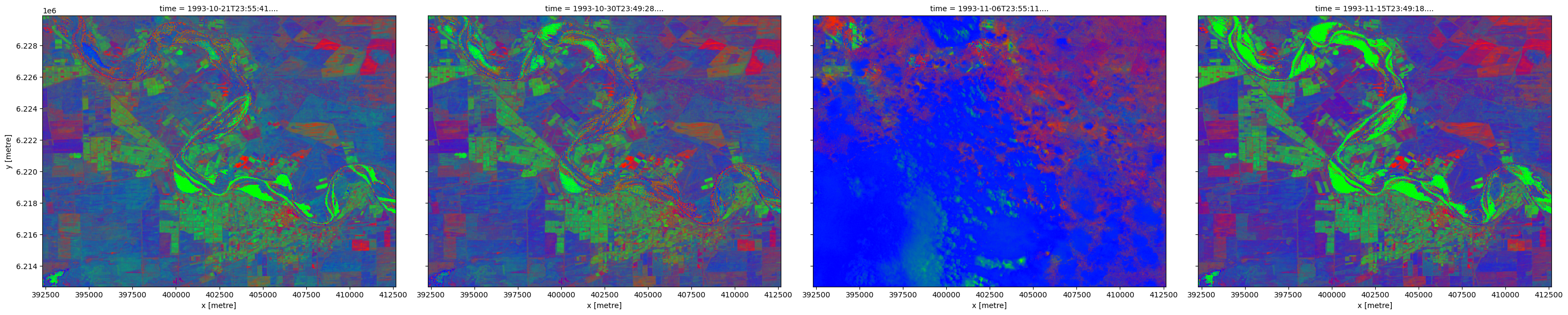
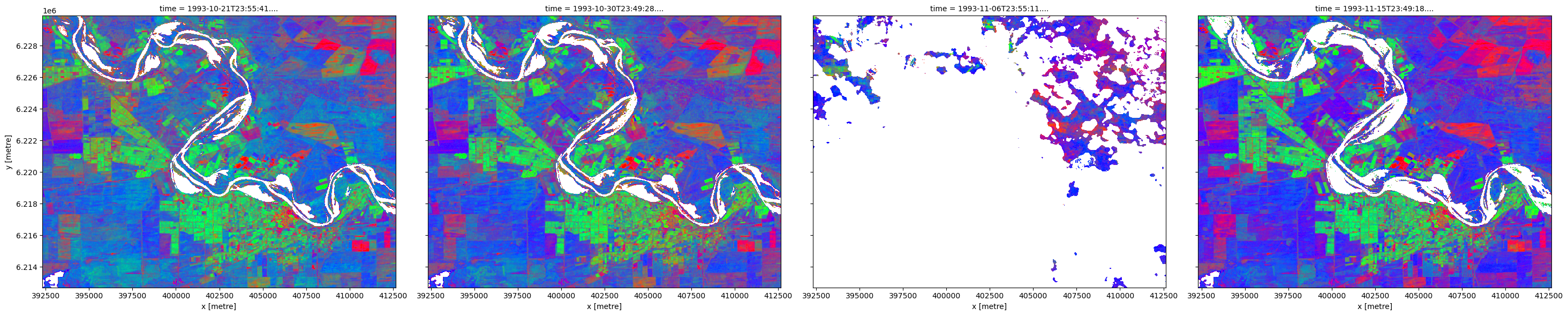
We can plot each FC variable in our dataset (i.e. ['bs', 'pv', 'npv']) using the rgb function. This will create a false colour view of the data where shades of green, blue and red represent varying proportions of vegetation and bare soil cover:

• Green: green vegetation (pv)

• Blue: brown (i.e. ‘non-green’) vegetation (npv)

• Red: bare soil (bs)

The resulting images show agricultural fields containing high proportions of green vegetation cover, surrounded by areas dominated by brown vegetation and bare soil. Note that the third image contains dense clouds which are erroneously mapped as non-growing vegetation.

Note: Fractional cover values range between 0 and 100%, but due to model uncertainties and the limitations of the training data, some areas may show cover values in excess of 100%. These areas can either be excluded or treated as equivalent to 100%.

# Plot DEA Fractional Cover data as a false colour RGB image
rgb(fc, bands=['bs', 'pv', 'npv'], col='time')

We can also visualise the ‘unmixing error’ (ue) for each of our DEA Fractional Cover observations. High unmixing error values (bright colours below) represent areas of higher model uncertainty (e.g. areas of water, cloud, cloud shadow or soil types/colours that were not included in the model training data). This data can be useful for removing uncertain pixels from an analysis.

In this example, wet pixels associated with a river have relatively high unmixing errors.

# Plot unmixing error using `robust=True` to drop outliers and improve contrast
fc.ue.plot(col='time', robust=True, size=5)

<xarray.plot.facetgrid.FacetGrid at 0x7f80688572b0>

Note: For more technical information about the accuracy and limitations of DEA Fractional Cover, refer to the Details tab of the official Geoscience Australia DEA Fractional Cover product description.

Example application: tracking changes in vegetation cover and bare soil over time

The following section will demonstrate a simple analysis workflow based on DEA Fractional Cover. In this example, we will process our loaded FC data so that we can consistently track the changing proportions of green vegetation, brown vegetation and bare soil over time.

Setting nodata

As the first step in our analysis, we need to set nodata pixels to NaN. This ensures that missing data is dealt with correctly in any future calculations.

# Replace all nodata values with `NaN`
fc = masking.mask_invalid_data(fc)

Applying a cloud and water mask

In the images we plotted earlier, you may have noticed the third panel is affected by cloud. This can cause the fractional cover algorithm to produce misleading results. FC will also produce poor results over water, causing erroneous values for green vegetation to appear within wet pixels (e.g. the fourth panel above).

To track FC reliably over time, we need to remove these potentially inaccurate pixels. One of the easiest ways to do this is to load data from the DEA Water Observations product that identifies wet and unclear pixels (e.g. cloud or cloud shadow) in the landscape.

In the next cell, we load DEA Water Observations data into the extents of our DEA Fractional Cover data using dc.load()’s like argument.

Note: For more details about loading data, refer to the Introduction to loading data notebook.

# Load DEA Water Observations data from the datacube
wo = dc.load(product='ga_ls_wo_3',
             group_by='solar_day',
             fuse_func=wofs_fuser,
             like=fc)

# Plot the loaded water observations
plot_wo(wo.water, col='time', size=5)

<xarray.plot.facetgrid.FacetGrid at 0x7f7dff222100>

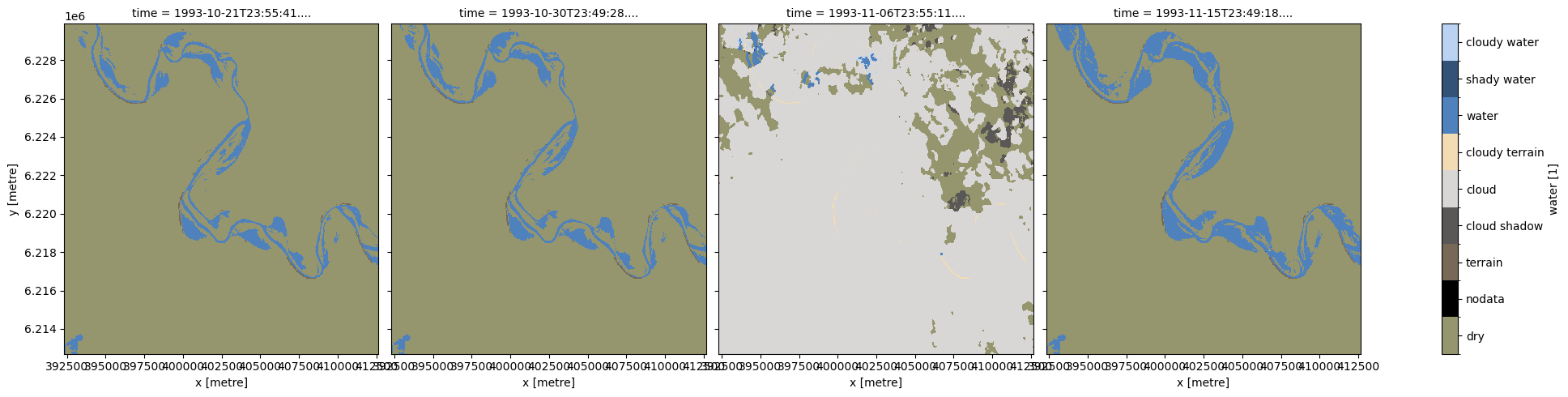
This plot shows that all images contain water, and the third image contains large amounts of cloud and cloud shadow. To remove these pixels, we first create a binary mask where True (yellow) represents clear and dry pixels, and False (purple) represents wet, cloudy or shadowy pixels.

Note: For a detailed guide to using DEA Water Observations data to mask data, see the DEA Water Observations notebook.

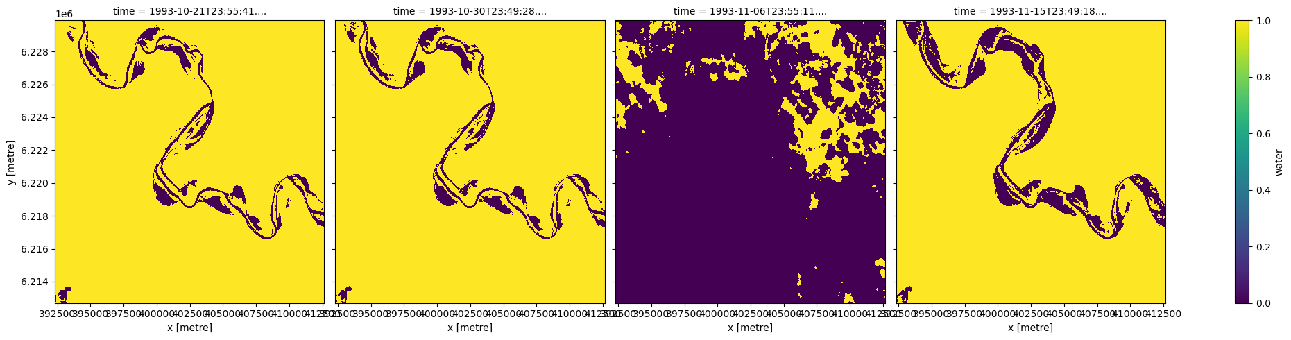
# Keeping only dry, non-cloudy pixels
wo_mask = masking.make_mask(wo.water, dry=True)
wo_mask.plot(col='time', size=5)

<xarray.plot.facetgrid.FacetGrid at 0x7f7dfe1c0640>

Using this mask, we can now remove any wet and unclear pixels from our original DEA Fractional Cover data. Note that these pixels now appear white as they have been replaced with NaN.

# Set any unclear or wet pixel to `NaN`
fc_masked = fc.where(wo_mask)

# Plot the masked fractional cover data
rgb(fc_masked, bands=['bs', 'pv', 'npv'], col='time')

Dropping poorly observed scenes

In the image above, we can see that the third observation was mostly obscured by cloud, leaving very little usable data. So that this doesn’t lead to unrepresentative statistics, we can keep only observations that had (for example) less than 50% nodata pixels.

# Calculate the percent of nodata pixels in each observation
percent_nodata = fc_masked.pv.isnull().mean(dim=['x', 'y'])

# Use this to filter to observations with less than 50% nodata
fc_masked = fc_masked.sel(time=percent_nodata < 0.5)

# The data now contains only three observations
fc_masked

<xarray.Dataset>
Dimensions:      (time: 3, y: 573, x: 678)
Coordinates:
  * time         (time) datetime64[ns] 1993-10-21T23:55:41.593257 ... 1993-11...
  * y            (y) float64 6.23e+06 6.23e+06 6.23e+06 ... 6.213e+06 6.213e+06
  * x            (x) float64 3.923e+05 3.924e+05 ... 4.126e+05 4.126e+05
    spatial_ref  int32 32754
Data variables:
    bs           (time, y, x) float64 16.0 19.0 16.0 24.0 ... 23.0 26.0 13.0
    pv           (time, y, x) float64 51.0 52.0 53.0 52.0 ... 26.0 20.0 31.0
    npv          (time, y, x) float64 32.0 27.0 29.0 23.0 ... 50.0 53.0 55.0
    ue           (time, y, x) float64 13.0 13.0 12.0 12.0 ... 11.0 11.0 13.0
Attributes:
    crs:           EPSG:32754
    grid_mapping:  spatial_ref

xarray.Dataset

• Dimensions:
  • time: 3
  • y: 573
  • x: 678
• Coordinates: (4)
  • time
    (time)
    datetime64[ns]
    1993-10-21T23:55:41.593257 ... 1...

    units :

    seconds since 1970-01-01 00:00:00

    array(['1993-10-21T23:55:41.593257000', '1993-10-30T23:49:28.344073000',
           '1993-11-15T23:49:18.275417000'], dtype='datetime64[ns]')

  • y
    (y)
    float64
    6.23e+06 6.23e+06 ... 6.213e+06

    units :

    metre

    resolution :

    -30.0

    crs :

    EPSG:32754

    array([6229875., 6229845., 6229815., ..., 6212775., 6212745., 6212715.])

  • x
    (x)
    float64
    3.923e+05 3.924e+05 ... 4.126e+05

    units :

    metre

    resolution :

    30.0

    crs :

    EPSG:32754

    array([392325., 392355., 392385., ..., 412575., 412605., 412635.])

  • spatial_ref
    ()
    int32
    32754

    spatial_ref :

    PROJCS["WGS 84 / UTM zone 54S",GEOGCS["WGS 84",DATUM["WGS_1984",SPHEROID["WGS 84",6378137,298.257223563,AUTHORITY["EPSG","7030"]],AUTHORITY["EPSG","6326"]],PRIMEM["Greenwich",0,AUTHORITY["EPSG","8901"]],UNIT["degree",0.0174532925199433,AUTHORITY["EPSG","9122"]],AUTHORITY["EPSG","4326"]],PROJECTION["Transverse_Mercator"],PARAMETER["latitude_of_origin",0],PARAMETER["central_meridian",141],PARAMETER["scale_factor",0.9996],PARAMETER["false_easting",500000],PARAMETER["false_northing",10000000],UNIT["metre",1,AUTHORITY["EPSG","9001"]],AXIS["Easting",EAST],AXIS["Northing",NORTH],AUTHORITY["EPSG","32754"]]

    grid_mapping_name :

    transverse_mercator

    array(32754, dtype=int32)

• Data variables: (4)
  • bs
    (time, y, x)
    float64
    16.0 19.0 16.0 ... 23.0 26.0 13.0

    units :

    percent

    nodata :

    255

    crs :

    EPSG:32754

    grid_mapping :

    spatial_ref

    array([[[16., 19., 16., ..., 40., 38., 41.],
            [21., 22., 19., ..., 40., 37., 39.],
            [22., 24., 20., ..., 28., 28., 25.],
            ...,
            [nan, nan, nan, ..., 12., 17., 18.],
            [nan, nan,  3., ..., 15., 16., 12.],
            [nan, 25., 13., ..., 17., 18., 13.]],
    
           [[ 6.,  2.,  9., ..., 39., 45., 41.],
            [ 8.,  7.,  5., ..., 44., 37., 36.],
            [ 6.,  4.,  2., ..., 28., 30., 31.],
            ...,
            [nan, nan, nan, ..., 21., 20., 21.],
            [nan, nan, 59., ..., 26., 21., 20.],
            [18., 30., 26., ..., 28., 21., 17.]],
    
           [[12., 10., 11., ..., 42., 39., 46.],
            [18.,  8.,  7., ..., 39., 41., 42.],
            [19., 12.,  5., ..., 33., 34., 35.],
            ...,
            [nan, nan, nan, ..., 18., 25., 25.],
            [nan, nan,  4., ..., 15., 25., 12.],
            [nan,  0., 20., ..., 23., 26., 13.]]])

  • pv
    (time, y, x)
    float64
    51.0 52.0 53.0 ... 26.0 20.0 31.0

    units :

    percent

    nodata :

    255

    crs :

    EPSG:32754

    grid_mapping :

    spatial_ref

    array([[[51., 52., 53., ..., 24., 23., 22.],
            [51., 52., 53., ..., 24., 21., 23.],
            [51., 54., 52., ..., 27., 24., 25.],
            ...,
            [nan, nan, nan, ..., 33., 33., 31.],
            [nan, nan,  5., ..., 32., 28., 38.],
            [nan,  7., 14., ..., 29., 28., 34.]],
    
           [[59., 64., 61., ..., 24., 23., 21.],
            [57., 62., 64., ..., 24., 23., 23.],
            [55., 63., 73., ..., 28., 24., 23.],
            ...,
            [nan, nan, nan, ..., 29., 30., 30.],
            [nan, nan, 10., ..., 27., 27., 29.],
            [15.,  9., 10., ..., 26., 22., 30.]],
    
           [[56., 58., 62., ..., 22., 23., 21.],
            [56., 56., 66., ..., 21., 23., 22.],
            [51., 60., 55., ..., 19., 20., 19.],
            ...,
            [nan, nan, nan, ..., 28., 27., 25.],
            [nan, nan,  0., ..., 32., 23., 34.],
            [nan,  6.,  8., ..., 26., 20., 31.]]])

  • npv
    (time, y, x)
    float64
    32.0 27.0 29.0 ... 50.0 53.0 55.0

    units :

    percent

    nodata :

    255

    crs :

    EPSG:32754

    grid_mapping :

    spatial_ref

    array([[[32., 27., 29., ..., 35., 37., 35.],
            [26., 25., 27., ..., 35., 40., 36.],
            [25., 21., 26., ..., 45., 46., 48.],
            ...,
            [nan, nan, nan, ..., 54., 49., 49.],
            [nan, nan, 92., ..., 52., 54., 49.],
            [nan, 66., 71., ..., 52., 53., 52.]],
    
           [[34., 33., 29., ..., 35., 31., 36.],
            [34., 30., 30., ..., 31., 38., 39.],
            [38., 31., 24., ..., 43., 44., 44.],
            ...,
            [nan, nan, nan, ..., 48., 49., 47.],
            [nan, nan, 30., ..., 46., 51., 50.],
            [66., 61., 63., ..., 44., 55., 51.]],
    
           [[31., 30., 25., ..., 34., 36., 32.],
            [25., 35., 25., ..., 38., 35., 35.],
            [29., 26., 38., ..., 47., 45., 45.],
            ...,
            [nan, nan, nan, ..., 53., 46., 49.],
            [nan, nan, 96., ..., 52., 51., 53.],
            [nan, 94., 71., ..., 50., 53., 55.]]])

  • ue
    (time, y, x)
    float64
    13.0 13.0 12.0 ... 11.0 11.0 13.0

    units :

    1

    nodata :

    255

    crs :

    EPSG:32754

    grid_mapping :

    spatial_ref

    array([[[13., 13., 12., ...,  9.,  9.,  8.],
            [12., 14., 14., ...,  9.,  9.,  9.],
            [12., 13., 14., ..., 10., 10., 10.],
            ...,
            [nan, nan, nan, ..., 14., 13., 13.],
            [nan, nan, 20., ..., 13., 12., 14.],
            [nan, 19., 12., ..., 12., 12., 14.]],
    
           [[15., 15., 16., ...,  9.,  9.,  8.],
            [15., 16., 18., ...,  8.,  9.,  9.],
            [14., 16., 18., ...,  9.,  9.,  9.],
            ...,
            [nan, nan, nan, ..., 12., 12., 12.],
            [nan, nan, 19., ..., 12., 11., 13.],
            [26., 19., 12., ..., 11., 11., 13.]],
    
           [[13., 14., 13., ...,  9.,  9.,  8.],
            [12., 15., 16., ...,  8.,  9.,  8.],
            [11., 14., 16., ...,  9.,  9.,  9.],
            ...,
            [nan, nan, nan, ..., 12., 12., 12.],
            [nan, nan, 21., ..., 12., 11., 13.],
            [nan, 20., 11., ..., 11., 11., 13.]]])

• Attributes: (2)

  crs :

  EPSG:32754

  grid_mapping :

  spatial_ref

Calculating average fractional cover over time

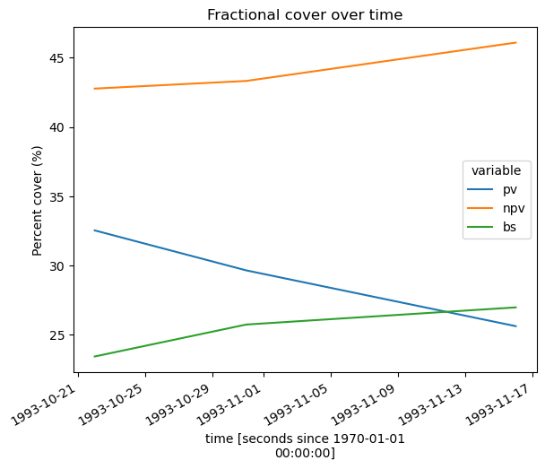
Now that our FC data has had nodata values and cloud, shadow and water pixels set to NaN and we have dropped unrepresentative observations, we can reliably track how average proportions of green and brown vegetation and bare soil have changed over time across our entire study area. We can then plot this as a line chart, showing that green vegetation (pv) has consistently decreased over time at this location, and brown vegetation (npv) and bare soil (bs) have increased.

# Calculate average fractional cover for `bs`, `pv` and `npv` over time
fc_through_time = fc_masked[['pv', 'npv', 'bs']].mean(dim=['x', 'y'])

# Plot the changing proportions as a line graph
fc_through_time.to_array().plot.line(hue='variable', size=5)
plt.title('Fractional cover over time')
plt.ylabel('Percent cover (%)');

---

Additional information

License: The code in this notebook is licensed under the Apache License, Version 2.0. Digital Earth Australia data is licensed under the Creative Commons by Attribution 4.0 license.

Contact: If you need assistance, please post a question on the Open Data Cube Slack channel or on the GIS Stack Exchange using the open-data-cube tag (you can view previously asked questions here). If you would like to report an issue with this notebook, you can file one on GitHub.

Last modified: December 2023

Compatible datacube version:

print(datacube.__version__)

1.8.9

Tags

Tags: NCI compatible, sandbox compatible, DEA products, ga_ls_fc_3, ga_ls_wo_3, rgb, plot_wo, fractional cover