Open Data Cube Workshop Material 
Compatibility: Notebook currently compatible with the
DEA SandboxenvironmentsPrerequisites: Users will benefit from having some experience with Python code prior to participation in this workshop
Introduction
These materials will introduce working with Digital Earth Australia (DEA) data in the DEA Sandbox environment for the Open Data Cube (ODC). The tutorial is broken into the following sections:
Getting started: Accessing the Sandbox
Jupyter Notebooks: What are they and how to use them?
Using interactive notebooks: Run a simple interactive notebook to perform a temporal analysis using DEA data
Do it yourself: Run and modify Python code to load, analyse and visualise data
Build it yourself: Explore the dea-notebooks code repository and build your own notebooks to answer specific analysis questions.
Learning more: How to continue exploring DEA data and resources
At the end of the tutorial you will know how to use a Jupyter Notebook in conjunction with the ODC to access and analyse Earth observation data. The tutorial should take around two hours to complete.
Notes for taking the workshop:
It’s a good idea to read this document from within the DEA Sandbox. Navigate to it at “Beginners_guide/Guided_tutorial.ipynb.”
For each notebook that you run, you should clear the example output by going to “Edit” > “Clear All Outputs.”
1. Getting started
The DEA Sandbox is a learning and analysis environment for getting started with Digital Earth Australia and the Open Data Cube. It includes sample data and Jupyter notebooks that demonstrate the capability of the Open Data Cube.
Sign up for a DEA Sandbox Account
The DEA Sandbox uses requires you to create an account to log in. Please visit https://app.sandbox.dea.ga.gov.au/ to sign up for a new account (a verification code will be sent to the email address you register with), or log in if you already have one.
Accessing the DEA Sandbox
After signing into the DEA Sandbox, your Jupyter environment will be created and you should see a loading screen while the system is working to prepare the environment.
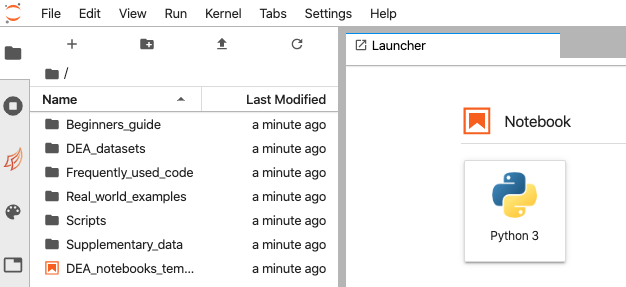
Once signed in, the JupyterLab homepage should appear. The JupyterLab interface consists of the main work area (right-hand panel), the left sidebar (containing a file browser and other useful features), and a menu bar along the top:
2. Jupyter Notebooks
Jupyter is an interactive coding environment that allows you to create and share documents, as Jupyter Notebooks, that contain live code, equations, visualizations and narrative text. Uses include: data cleaning and transformation, numerical simulation, statistical modeling, data visualization, machine learning, and much more.
The name ‘Jupyter’ comes from Julia, Python and R, which are all programming languages that are used in scientific computing. Jupyter started as a purely Python-based environment called iPython, but there has been rapid progress over the last few years, and now many large organisations like Netflix are using the system to analyse data.
As the ODC is a Python library, the workshop will cover working with Earth observation data in Python-based notebooks.
Getting started with Jupyter
The first exercise is to explore and understand some key features of the Jupyter notebook, including how to run cells containing code, and edit documentation.
Click the link to run the following notebook and return here when you have worked through the examples:
3. Using interactive notebooks
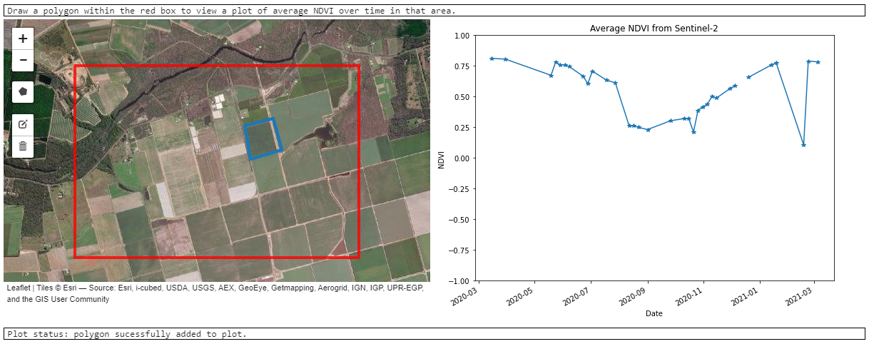
A major feature of the Open Data Cube approach is its spatiotemporal data richness and searchability. The following notebook has been designed as an application, with almost all of the code stored in the background as a function. Its purpose is to show users the temporal data richness that is stored in the DEA archive. In this notebook, the most recent 12 months worth of Sentinel 2 data is loaded over a predetermined location. Users can select small sub-locations to compare changes in the relative greenness (NDVI) response over time.
Click the link to run the following notebook and return here when you have worked through the examples:
4. Do it yourself
This activity uses a code-based Jupyter notebook to demonstrate how the ODC Python API works. This example includes the following analysis steps:
Picking a study site in Australia
Loading satellite data for that area
Plotting red, green and blue satellite bands as a true colour image
Using a vegetation index to calculate the “greenness” of an image
Exporting your data to a raster file
Next steps
Once you have run the notebook in its entirety, return to the top and experiment with changing some of the variables. For example, consider setting a new study location, and/or changing the time period of the analysis.
Click the link to run the following notebook and return here when you have worked through the examples:
5. Build it yourself
For the next excercise, we will build a new analysis focused around a specific scientific question:
Monitor how waterbodies in Australia have changed over time using satellite data.
Choose one of the following options depending on difficulty:
Intermediate level: Update the basic analysis notebook to study changes in water over time
Starting at the top of the Performing a basic analysis notebook, modify the notebook to change the analysis to focus on monitoring changes in water over time. This could involve:
Changing the study area to a location with a waterbody (e.g. Canberra’s Lake Tuggeranong, or Lake Menindee in western New South Wales)
Change the Normalised Difference Vegetation Index (NDVI) used in the notebook to a new index that is better for monitoring water. For example, the Normalised Difference Water Index (NDWI) that is used to monitor changes related to water content in water bodies:

Plot the output water index results for different timesteps to compare how distributions of water have changed over time.
Advanced level: Build a new analysis from scratch
Starting from a blank notebook (hint), build a new analysis from scratch using content from the Performing a basic analysis notebook, and code from other notebooks in the Digital Earth Australia Notebooks repository. For example, this could involve:
Using the
load_ardfunction to load cloud-free Landsat or Sentinel-2 imagery (see the Using load_ard notebook)Calculating a water index (e.g. Normalised Difference Water Index or NDWI) using the
calculate_indicesfunction (see the Calculating_band_indices notebook)Plot the output water index results for different timesteps to compare how distributions of water have changed over time.
Tips
You can view multiple notebooks simultaneously in Jupyter Lab. Simply click and drag your notebook tab to the right hand side of your screen for a side by side view.
All the code in this repository is open source and we encourage code recycling to fit your needs. Therefore, you can copy/paste cells between notebooks by right-clicking inside a cell, selecting
Copy Cellsand then navigating to your desired paste-location and right click any cell then selecting ‘Paste Cells Below’
6. Learning more
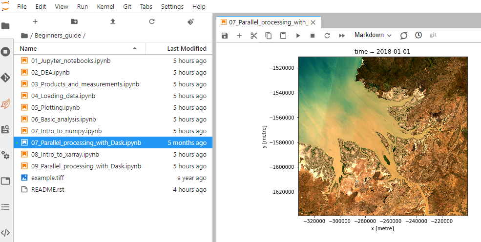
For a more detailed introduction to Digital Earth Australia and the Open Data Cube, we recommend running the entire set of Beginner’s Guide notebooks located in this folder, starting with Performing a basic analysis and continuing on to Parallel processing with Dask.ipynb.
You can now join more advanced users in exploring:
The “DEA products” directory in the repository, where you can explore DEA products in depth.
The “How_to_guides” directory, which contains a recipe book of common techniques and methods for analysing DEA data.
The “Real_world_examples” directory, which provides more complex workflows and analysis case studies focused on answering real-world scientific and management problems using the Open Data Cube.
Additional information
License: The code in this notebook is licensed under the Apache License, Version 2.0. Digital Earth Australia data is licensed under the Creative Commons by Attribution 4.0 license.
Contact: If you need assistance, please post a question on the Open Data Cube Discord chat or on the GIS Stack Exchange using the open-data-cube tag (you can view previously asked questions here). If you would like to report an issue with this notebook, you can file one on
GitHub.
Last modified: April 2023
Tags
Tags: sandbox compatible, beginners guide, ODC workshop